Market In Motion

HOUSTON–After an exceptionally mild winter nearly derailed the U.S. natural gas market earlier this year, the supply and demand balance ended the 2016-17 withdrawal season in a much more bullish position. In fact, at the start of the 2016 injection season last spring, the U.S. natural gas market was exiting an extremely bearish winter, the storage inventory was nearly 500 billion cubic feet higher, and Henry Hub futures prices were trading more than $1 an MMBtu lower. The overarching sentiment was that prices would have to remain low to balance the market.

The industry is exiting an almost equally mild winter this spring, but a combination of lower production and higher exports has drawn storage to a range well within the five-year average, and the question occupying everyone’s minds is how bullish this year’s market can get.

The April 2017 Henry Hub natural gas futures contract expired on March 29 at $3.175/MMBtu on the Chicago Mercantile Exchange/New York Mercantile Exchange, which was nearly $1.30 (67 percent) higher than the April 2016 contract settlement of $1.90/MMBtu and about $0.55 higher than the March 2017 contract settlement. Yet, with the end-of-March storage inventory still 265 Bcf higher than the five-year average and production growth on the horizon, this year’s market remains susceptible to downside risk if incremental demand fails to show up. So how did we get here, and what lies ahead?

The market exited the first-quarter 2016 from one of the most bearish winters on record, with more than an 800 Bcf storage “surplus” compared with the five-year average and 1 trillion cubic feet more than the prior year. Nevertheless, by year’s end, the market not only had managed to wipe out the surplus, but also ended net short on supply for the year and prices were approaching $4.00 an MMBtu in December. Both the supply and demand sides of the balance equation contributed to this remarkable shift.

In 2016, total supply (including imports) averaged 77.5 Bcf/d, down 1.3 Bcf/d from 2015. Total demand (including exports) averaged 78.5 Bcf/d, up 1.3 Bcf/d year over year. So the resulting net balance of supply minus demand went from positive 1.6 Bcf/d in 2015 to negative 1.0 Bcf/d in 2016. In other words, the gas supply and demand balance averaged 2.6 Bcf/d “shorter supply” in 2016 versus 2015.

On the supply side, 2016 U.S. gas production contracted by 1.8 Bcf/d, posting the decade’s first year-on-year decline. Lower rig counts finally caught up to producers that had, until then, managed to maintain or grow production by drilling better and faster with fewer rigs, while Northeast capacity constraints also helped flatten Marcellus Shale growth.

Tightening the balance further was the fact that demand rose about as much as production fell. While mild weather stunted residential and commercial heating demand, demand in almost all other sectors climbed–to record levels in many cases–spurred by lower prices and export capacity additions. A standout was the rapid rise of new demand from liquefied natural gas exports, which commenced in February 2016 and quickly grew to more than 1 Bcf/d by the start of 2017.

Bullish Balance

Given the balance, 2016 ended on a bullish note and prices seemed to be on their way to $4.00 an MMBtu for the first time in two years. That did not last long, however. The bullish sentiment was squashed by extremely mild weather in the first quarter of 2017, which proved even milder than in 2016. But the bulls have hung on nevertheless. While prices retreated in the face of unseasonable January and February temperatures, they have remained in the $3.00 an MMBtu range heading into the spring/summer refill season. That is because the same bullish balance that helped prevent storage constraints in 2016 still lurks beneath all the mild weather.

In late February, supply was 3.5 Bcf/d longer year to date versus the same period in 2016. While supply was averaging 3.1 Bcf/d lower (primarily lower production) demand was down even more–an astonishing 6.6 Bcf/d year on year–resulting in the extremely bearish balance of 3.5 Bcf/d. But when the January and February 2017 residential/commercial demand volumes are substituted with 2016 or five-year average residential/commercial volumes for the same period, a very different balance emerges: one that is short on supply by close to 2.0 Bcf/d. In other words, strip away the bearish effects of the warm winter weather and assume even average temperatures and the supply/demand balance easily flips from net bearish to net bullish.

Moreover, since late February, weather has turned less bearish, and that underlying bullishness is now apparent. A look at the year-to-date balance at the end of March, for instance, shows a supply shift within one month’s time from being 3.5 Bcf/d long in February to very slightly (0.1 Bcf/d) short. Looking at the November 2016-March 2017 withdrawal season as a whole, the market averaged 3.0 Bcf/d shorter supply compared with the 2015-16 withdrawal season. That has meant withdrawals have been sufficiently strong to leave the storage inventory lower than where it was at this time last year, despite starting this past winter at a record high and despite the lower residential/commercial heating demand.

The Energy Information Administration’s official end-of-March storage inventory was 2.05 Tcf. That was 430 Bcf (17 percent) lower than at the end of last winter, but still 260 Bcf (11 percent) higher than the five-year average. With injection season officially under way since April 1 (even though the market saw the first-ever storage injection in the month of February this year), the question becomes what the current balance and storage level mean for storage and prices during the April-to-October injection season. Will the year-on-year deficit in storage provide sufficient cushion, or is there still a chance that storage can test capacity and sink prices again?

Supply/Demand Scenarios

The supply/demand balance determines the pace of injections, so before we can consider storage scenarios, we must first look at possible supply/demand balance scenarios. To arrive at some plausible supply/demand scenarios for the 2017 injection season, some assumptions are necessary about each component based on historical data, holding a few variables constant for simplicity’s sake. For example, each of the first set of scenarios assumed that production would stay flat to the 30-day average of 70.6 Bcf/d, which actually would be a decline of about 0.4 Bcf/d from the 2016 injection season.

Since imports display seasonality relative to U.S. demand, the average import volumes during the 2016 injection season were used instead of the most recent 30 days. Canadian imports averaged 6.1 Bcf/d last year, while LNG send-out (such as pipeline receipts of regasified LNG) averaged a paltry 0.2 Bcf/d. On the demand side, exports are growing rapidly and are expected to continue increasing. However, for these scenarios, we assume they remain flat to the most recent 30-day average, which comes to 4.0 Bcf/d for exports to Mexico and 1.9 Bcf/d for pipeline deliveries to Cheniere Energy’s Sabine Pass LNG export facility.

That leaves U.S. consumption for power generation, industrial plants and residential/commercial usage, all of which are driven to varying degrees by the perennial wild card in any supply/demand forecast: weather. For these components combined, four demand scenarios were considered for the 2017 injection season:

• Flat compared with the 2016 injection season;
• Tracking the three-year highs for each month of injection season, which follows 2016 numbers except for a spike that occurred in October 2015;
• Equal to the three-year average; and
• Regressing to the three-year monthly average lows for the season, which corresponds to 2014 levels.

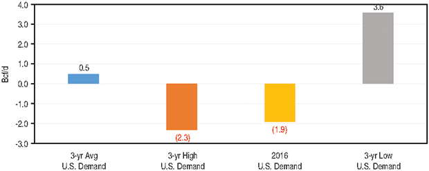
FIGURE 1

Modeled Scenarios for Year-Over-Year Changes
In Supply/Demand Balance
(2017 Injection Season)

Source: All images courtesy of RBN Energy LLC. Historical supply and demand data from RBN Energy’s Natgas Billboard daily report.

Figure 1 shows the year-on-year changes, or how much longer or shorter the market will be this injection season versus 2016, according to these assumptions and demand scenarios. If production, exports and imports all stay flat, but demand drops to the three-year average (a full 2.4 Bcf/d below last year), market supply will be 0.5 Bcf/d longer than last year (blue bar). If demand reverts back to three-year lows for each month, the balance will be 3.6 Bcf/d longer than last year (gray bar). But the scenarios also show that if U.S. demand manages to merely sustain last year’s injection season, the outcome will be a market that is nearly 2.0 Bcf/d tighter (yellow bar). And if demand replicates the three-year highs for each month of injection season, the balance will be 2.3 Bcf/d tighter (orange bar).

These scenarios assume flat production and exports, but we know Baker Hughes shows gas rig counts climbing from 88 in the first week of April 2016 to 165 in the same week this year. It is hard to predict how fast production will bounce back, but the groundwork has been laid for some growth in 2017, especially given that the price curve also is more supportive. We also know that significant export capacity volumes have been added since last summer, both to Mexico and to the Sabine Pass LNG facility, suggesting there is a good chance exports are primed to grow as well.

Turning The Market Short

FIGURE 2

Demand, Production and Export Scenarios
On Year-Over-Year Supply/Demand Balance
(2017 Injection Season)

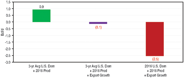
The scenarios in Figure 2 consider how these factors impact the natural gas balance. To start with production growth, taking the three-year average demand scenario but assuming production returns to the 2016 summer average of 71 Bcf/d (an 0.4 Bcf/d increase versus the current 30-day average), yields a balance nearly 1.0 longer on supply versus 2016 (green bar), which no doubt will have a bearish impact on storage and the price curve.

However, as the purple bar shows, all it takes is some export demand to turn the market short. In this scenario, U.S. demand remains at the three-year average level and production returns to the 2016 level, but export demand increases by a total of 0.6 Bcf/d (0.3 Bcf/d each from LNG and Mexican exports). That is not much of a stretch, considering Sabine Pass was approved to start its third liquefaction train and has begun commissioning activity for a fourth.

In addition, the market will have more than 3.0 Bcf/d of new pipeline capacity for exports to Mexico this summer, including Energy Transfer Partners’ 1.4-Bcf/d Trans-Pecos Pipeline, which began service on March 31. Flows on this new export capacity are not expected to grow nearly as fast as pipeline capacity is being added, given that demand and connectivity across the border in Mexico have yet to catch up. However, it is safe to assume that it will grow, even if gradually.

Based on these assumptions, the market will average 0.1 Bcf/d short versus 2016, in spite of demand being 2.4 Bcf/d lower than last year. Then, if production remains at the 2016 level and exports increase 0.6 Bcf/d, while U.S. demand stagnates after last year’s record highs, supply will end at least 2.5 Bcf/d short (red bar) this year–a highly bullish prospect.

The take-away from these scenarios is that, unlike last year, production can grow and the balance still will tighten. Another way to look at it is that the scenarios imply U.S. consumption must drop considerably for the market to turn more bearish compared with 2016. And that is without even accounting for export demand growth, which is all but inevitable this year. But what do these various scenarios mean for the storage inventory, and by extension, for prices?

Gas Storage Impact

Since storage activity, including injections and withdrawals, is more or less the net effect of supply minus demand, the daily balances from each of these supply/demand scenarios can be carried forward through the 214 days of the storage injection season to get the net change in storage over that time.

FIGURE 3

Storage Injection By Season
(Historical versus 2017 Modeled Scenarios)

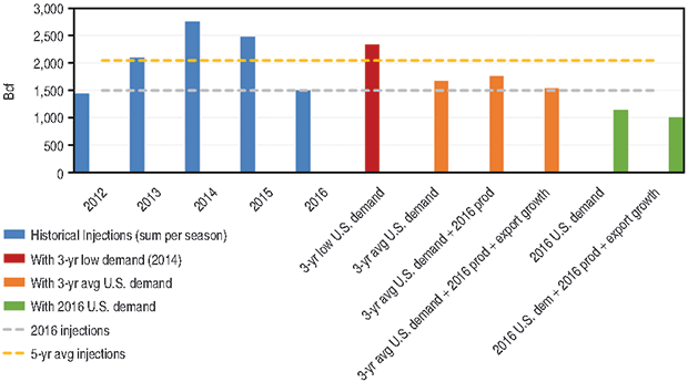
Figure 3 summarizes those results. The blue bars show the historical sum of injections for April through October since 2012 based on historical EIA data. The average of the blue bars is 2.048 Tcf (yellow dashed line), which compares with last year’s total injections of 1.5 Tcf (gray dashed line). The remaining bars show the total injections that will result from each of the aforementioned balance scenarios. For instance, if production and exports stay flat to the recent 30-day average and imports are flat to 2016 injection season levels, but demand drops to the three-year low (for example, ~5.0 Bcf/d lower than last year), injections will be close to a robust 2.3 Tcf (red bar), soaring above 2016 and also well above the five-year average.

Next, if we look at scenarios using three-year average U.S. consumption volumes (orange bars), injections will range from 1.5 Tcf to 1.8 Tcf at most. That is well below the five-year line, but potentially above 2016. Injections will land on the higher end of that range if no incremental demand materializes (left-most orange bar), and even more so if production rises to 2016 levels (middle orange bar). But they will come in on the lower end of the range (nearly flat with 2016) with 0.6 Bcf/d in export growth, even if production also grows (right-most orange bar).

If 2017 injection season consumption averages the 2016 level (green bars), which is essentially also the three-year high for seasonal demand, total injections will drop to near the 1.0 Tcf mark, well under both the five-year and year-ago levels. More specifically, it will be closer to 1.1 Tcf with no incremental export demand (left green bar) and slightly lower (1.0 Tcf) with export demand growth. And that will be true even if production returns to the 2016 level (right green bar).

Altogether, these scenarios suggest that unless production climbs substantially or U.S. consumption falls drastically from last year, injections are likely to be on the lower end of the spectrum. The bottom line for price direction, however, is where these injection scenarios leave the overall U.S. storage inventory next fall. To provide answers, inventory levels are projected through October based on the different modeled injection scenarios (Figure 4).

FIGURE 4

Gas Storage Inventories
(Historical versus 2017 Modeled Scenarios)

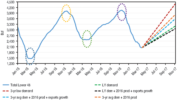
As the blue solid line shows, storage inventory started the 2015 injection season at the relatively low level of 1.5 Tcf (blue oval), but as production climbed, the market injected nearly 2.5 Tcf that summer. By November, storage had peaked above 4 Tcf for the first time (yellow oval). That record level was followed by the mild 2015-16 winter, which left the year-over-year inventory much higher at the start of the 2016 injection season (green oval).

However, record demand through much of the 2016 injection season suppressed injections to less than 1.5 Tcf. While the inventory peaked at a new record of 4.047 Tcf in November 2016 (purple oval), it was not by much considering how high the inventory had been seven months earlier.

End-Of-Season Inventory

Although 2016-17 winter weather was again mild, strong exports and lower production allowed the market to withdraw nearly 2 Tcf between Nov. 1 and March 31. With 2 Tcf in storage at the start of the 2017 injection season this spring, how likely is it that the storage inventory will again approach or exceed the 4.0 Tcf level by the start of the next winter heating season on Nov. 1, as it did the past two years? Based on our scenarios, not very.

The dashed lines on the right side of Figure 4 project inventory through October based on the modeled supply/demand and injection scenarios. Two of the projections assume U.S. consumption will drop to the three-year average (2.4 Bcf/d lower than 2016). One assumes production will rise modestly to 2016 levels, but exports will remain flat (orange dashed line). The other surmises that production will rise, but exports also will grow (blue dashed line). The resulting season-ending inventory projections range from 3.5 Tcf with incremental export demand to 3.8 Tcf without it. In all cases, the storage inventory at the end of the 2017 injection season is projected to be well below 4.0 Tcf.

If consumption during this year’s injection season tracks 2016’s record level, the implied injections will leave inventory close to 3.0 Tcf by autumn (the green and black dashed lines). In fact, the only modeled scenario that even approaches 4.0 Tcf is the low-demand case, in which U.S. consumption declines to a three-year low and exports do not grow (red dashed line). In that case, the inventory will end well above 4.0 Tcf. This is the most bearish scenario, but also the least likely, given the substantial new export capacity available heading into this injection season. In addition, if inventory begins to balloon, prices likely will be pressured to the point at which gas displaces more coal in the power sector, thereby stimulating consumption.

Considering that most of the scenarios lead to relatively bullish outcomes compared with last year, it is no wonder that $3.00 an MMBtu pricing has held in the futures curve, even as weather remains mild. That said, however, some curve balls still could knock the market off its generally bullish course. For instance, on the bearish side, production could roar back faster than expected in the second half of 2017. On the bullish side, exports or U.S. consumption also could grow more than assumed. What we do know from modeling these scenarios is that the year-on-year deficit in storage and the underlying supply/demand balance give the bulls an edge as the injection season gets into full swing.