Pressure Integrity Test Interpretation

HOUSTON–Formation pressure integrity tests (FPITs) are conducted immediately after drilling out a casing or liner shoe, and occasionally when additional formation has been exposed while drilling ahead, to verify the integrity of cement at a casing shoe, to determine the maximum equivalent circulating density (ECD) to which a shoe can be safely exposed, and to measure the stress state of the exposed formations for well planning and operations.

FPITs include jug tests, leak-off tests, formation integrity tests, breakdown tests, extended leak-off tests, and repeat extended leak-off tests. The critical operational decisions made directly from the results include the need for remedial cement operations, maximum mud weights that can be used to drill the next well section, minimum mud weights that can be used to prevent hole collapse, calibration factors for predicting fracture gradients, and the potential need for lost circulation mitigation strategies.

FIGURE 1

Typical FPIT Rig Up

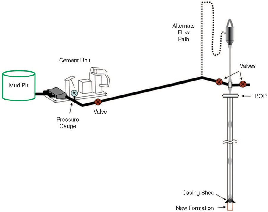
FPIT data interpretation techniques frequently focus on the point at which a fracture initiates, the point where unstable fracture growth begins, or the closure pressure of the fracture when pumping ceases. However, early pressure buildup behavior often is overlooked and can provide insights on the integrity of cement, the point of fracture initiation, the permeability of the formation being tested, the need for cement remediation, and the potential to increase fracture resistance using wellbore-strengthening techniques.

Figure 1 shows the general rig-up for an FPIT. The basic procedure consists of running a casing integrity test (CIT) before drilling out the cement at the shoe to establish the integrity of the casing and/or liner. Following the CIT, the cement inside the casing and rat hole is drilled out and three meters of fresh formation typically are drilled. The mud is conditioned through adequate circulation and the drill bit is pulled back into the casing to minimize any risk of sticking the downhole assembly while conducting the test.

The cement unit is connected to the drill pipe and/or annulus, and circulation is established. The annular or pipe rams are closed around the drill pipe, and mud is pumped down the drill pipe/choke line into the closed system while recording the pumped mud volume and the surface pressure until the target test pressure is achieved. The pumps then are shut down and pressure decay is monitored until the pressure stabilizes. The data are analyzed to determine whether a fracture was introduced, propagated or closed, and to quantify the associated pressures.

Fracture Initiation

To determine either the stress state of the exposed formation or the maximum ECD to which the formation at the shoe can be exposed safely, it is necessary to pressure the formation below the shoe until a fracture is induced. Figure 2 displays an idealized pressure response recorded while conducting a test. The leak-off pressure (LOP) is the point where a fracture initiates at the wellbore interface. If pressure increases above the LOP, stable fracture growth may occur until the peak or breakdown pressure is achieved, at which time unstable fracture growth will occur away from the well into regions of the formation undisturbed by drilling.

FIGURE 2

Idealized Example Pressure Response

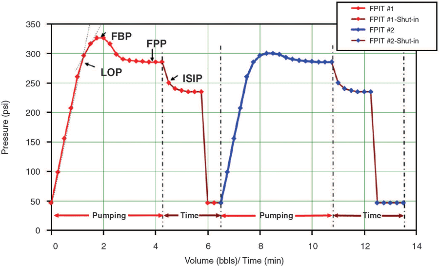
If pumping continues, the pressure should stabilize to the fracture propagation pressure. When pumping is finally halted, the pressure should drop immediately as friction pressure is removed from the well and the instantaneous shut-in pressure is observed. If well pressure is greater than the pressure required to hold the fracture open, the fracture will continue to grow until the pressure falls below the fracture closure pressure and the fracture closes.

The pressure may continue to decline after the fracture closes, if permeability is exposed in the well, and as mud and formation temperatures equilibrate. However, comparing surface and downhole data suggests that the pressure decline down hole is often not as marked as that seen at the surface. Some of the surface pressure drop may be a result of mud gelling effects.

Fracture closure pressure can be the most valuable piece of information from the test used to determine the stress state of the formation beyond the influence of the well. However, many operators resist pumping the amount of mud required to achieve fracture propagation pressure because of concern that the fracture may grow a significant distance and encounter lower-stressed rock, limiting the maximum mud weight that can be used to drill the next hole interval.

It is also important to identify the leak-off point, since it establishes the point at which a fracture starts (or at least where its growth is visible from the measurements), and in part, can be used to establish the maximum safe ECD. When combined with a repeat of the test, the leak-off point also can be used to estimate the formation’s tensile strength. It is described most frequently as the point where the trend of the pressure increase deviates from linearity.

In a significant number of tests, the pressure-volume trend prior to initiating a fracture is nonlinear. This can make it difficult to accurately identify the leak-off point. Modeling can be used to analyze the shape of the trend prior to fracture initiation, which then can aid greatly in understanding the behavior of the test (and accurately determining the fracture initiation pressure). The results of the modeling also can be used to understand the properties of the exposed formation and the potential for the presence of a channel behind the casing.

Pressure Buildup Model

A new model has been developed for predicting early pressure buildup behavior. The behavior of the pressure-volume curve (or compliance of the system) prior to fracture initiation is governed by a number of primary factors, including mud compressibility, casing expandability, cement compressibility, formation compressibility, air in lines, permeability losses, and channel volume.

A pressure-volume slope of the CIT is a direct measure of system compliance prior to drilling out the cement and the casing shoe, and exposing new formation. That compliance is a function of casing expandability, which also is a function of cement and rock compressibility and the fluid in the uncemented annuli. However, the dominant factor effecting system compliance in a CIT is the compressibility of the mud. Rather than break down the CIT slope into its various components, it is more convenient to work in terms of an apparent mud compressibility as defined by the CIT pressure-volume slope.

Depending on the well construction at the time of a test, actual mud compressibility (as an average of the temperature and pressure conditions of the entire mud column) can be expected to be as much as 15 percent less compressible than apparent mud compressibility. For all practical purposes, apparent mud compressibility backed out from the CIT will apply to the FPIT as well, assuming the basic mud properties have not changed significantly between the two tests. Adjusting from CIT to FPIT conditions needs to take into account the additional mud volume resulting from drilling out the cement to the casing shoe, drilling out the rat hole, and any new exposed hole.

The apparent mud compressibility is applied to the new system volume to get a first estimate of the expected pressure-volume slope for the FPIT. CIT pressure-volume responses should be linear. Apparent nonlinearity may occur as a result of variations in the pump rate or when there are leaks in the system. The effects of air trapped in the lines also may be observed, but those effects diminish quickly in the early stages of the test, and usually are unnoticeable over much of the CIT plot.

FIGURE 3

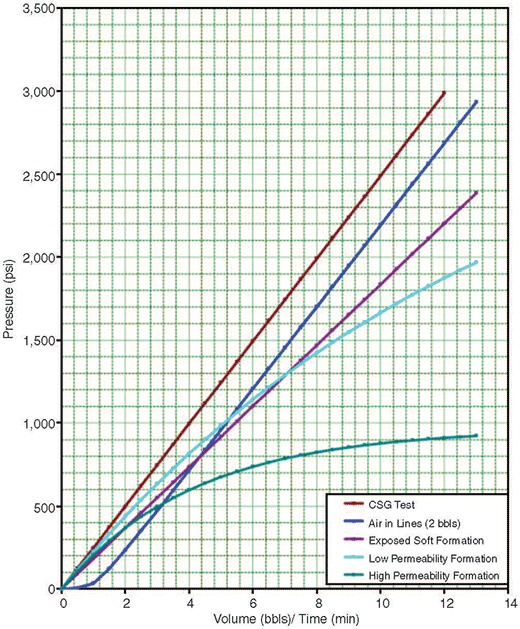
Example Modeled Responses

Using a series of equations, the model can be applied to determine the apparent mud compressibility, as well as the expected pressure-volume slope, for the FPIT. The actual FPIT slope often is compared in the first instance with the CIT slope. Where there is not a good match between the slopes, further investigation can be conducted by considering formation compressibility, air in lines, permeability losses, and potential channel volume properties. These properties can be adjusted to optimize the fit to observed data.

Figure 3 displays the expected generalized response to the model’s individual components. The casing test (brown curve) reflects the compression of the mud, and the expansion of the casing and cement as a function of applied pressure. The response should be linear. The slope decreases as the volume of the system increases, as additional new formations are exposed, or as the compressibility of the fluid increases.

When air is introduced into the system (usually while making connections between the cement unit and drill pipe) and is not circulated out, the response (blue curve) initially will be near-flat and then quickly curve upward to near-parallel to the casing test as the applied well pressure increases. As pressure is applied, the volume of air decreases. As mud is pumped, air is pushed down the hole, subjecting it to both the pressure of the column above and the applied surface pressure. Once subjected to sufficient pressure, the volume of the air becomes so small that its effect on the slope of the curve is negligible.

When any formation is exposed to the test, the formation will compress in response to the applied pressure, which will cause the linear slope of the purple curve in Figure 3 to decrease. The softer the formation (lower modulus) and the greater the exposed formation surface area, the more the slope of the line decreases. In most cases, the amount of change in wellbore volume is very small.

If a permeable formation is exposed below or behind casing during the test, fluid can be lost into the formation once well pressure is greater than formation pore pressure. The rate of loss is a function of formation permeability, the amount of exposed permeable surface area, and the difference between formation and well pressure. As the difference between well and formation pressure increases, the rate of loss will increase also, causing the slope of the line (light blue and green) to curve toward a lower slope. In high-permeability formations and high-differential pressures, it is possible for the slope to approach horizontal without introducing a fracture.

The model allows all of these effects to be taken into account simultaneously. There are other effects that may occur from time to time (e.g., movement of drill pipe, variations in pump speed, pump efficiency issues, and variations in fluid properties) that may impact the early curve behavior that the model does not address, but using the model can help identify those issues.

Basic Workflow

The basic workflow to model the pressure-volume response of an FPIT includes:

• Calculating apparent mud compressibility from the casing test;
• Calculating apparent mud response using the exposed volume at the time of the open-hole test;
• Calculating the formation compressibility response;
• Adjusting the amount of air in the lines to fit the early upward curvature;
• Adjusting the formation permeability parameters to fit the downward curvature; and
• Iteratively using air, channel size, and permeability parameters until a “best fit” is found to the measured data.

The casing test pressure-volume trend should form a linear line. Irregularities commonly exist at low pressure readings as the pumping unit operator brings the unit up to speed and adjusts the rate to the desired target. These fluctuations in rate produce variations in friction pressure that are most pronounced when observed with surface gauges, but are significantly lower when observed with downhole gauges.

A linear trend can be determined from the stable higher-pressure readings, and can be used to calculate apparent mud compressibility. This relationship also requires knowledge of the volume of the mud exposed to the casing test, which consists of the volume of the casing above the cement plug, the volume of the choke/kill line (if used), the volume of the surface plumbing between the well and the cement unit, and the volume and displacement of any drill pipe that may have been used during the test.

If the compressibility of the mud used during the open-hole test has been altered significantly from the mud used during the casing test, an alternative source for mud compressibility will be required. Most mud vendors are able to model the compressibility of their products for a given well configuration. If this is impossible, values from past experience can be used.

The pressure-volume response to the mud in the well at the time an FPIT is conducted also can be modeled. This calculation requires knowledge of the total volume of the system when the open-hole test is conducted, which will have changed from the volume present when the CIT was conducted. This volume can be estimated from assessing the casing volume, open-hole volume below the shoe, drill pipe displacement below the blowout preventer, drill pipe capacity above the BOP, the choke/kill line volume (if used), surface plumbing volume between the drill pipe and the cement unit, and any potential channel behind the casing exposed at the time of the test.

Once these inputs are known, the pressure change for each increment in the pumped mud volume can be calculated and compared with the measured response. If the volume of the system present during the CIT is less than the volume of the connected system present during the open-hole test, the slope of the open-hole test will be lower than the slope of the casing test.

If the volume of the system during the casing test is greater than the volume of the connected system in the open-hole test, the slope of the open-hole test will be higher than the slope of the casing test. The latter case can occur when significant casing volume is displaced by drill pipe during the open-hole test.

Modeling Responses

When a significant amount of soft formation surface area is exposed during the test, these formations can compress, increasing system volume and decreasing the slope of the pressure-volume curve. In most cases, the effect of formation compressibility is negligible. However, the impact could be noticeable if very soft formations are present, low-compressibility mud is being used, and a large surface area is exposed because of long open-hole sections below the shoe (or a large connected channel behind the casing). Formation compressibility often can be calculated from petrophysical log data or from correlations with effective stress.

The impact of mud compressibility, changes in hole volume, and the exposure of a compressible formation are all linear, hence not unique. Errors in evaluating one of these properties can be cancelled by an opposing error in assessing one of the other linear responses. However, the presence of permeability and air trapped in the lines are both nonlinear and produce a unique modeling response.

During the rig-up process, air can be trapped easily in surface lines. The compressibility of air is inversely proportional to absolute pressure. Air is highly compressible, compared with water-base or synthetic mud.

As mud is pumped into the system, the pressure increases and air is pushed down the well, further increasing the air pressure and proportionally decreasing the air volume. The effect is that air trapped in lines begins nearly flat and then curves upward rapidly, typically becoming indistinguishable by the time 100 psi is applied. Because the characteristic shape of the air in lines is so short lived, it is quite easy to fit by simply adding air to the model. The typical quantity encountered is usually on the order of a few tenths of a barrel.

The presence of permeability results in the loss of mud to the formation, which creates the downward curvature of the pressure-volume curve. This is the only attribute that creates downward curvature, so it is uniquely matched using permeability attributes. By adjusting the flow factor and pore pressure used to calculate the difference between well pressure and formation pore pressure, the fit of the downward curvature of the modeled data to the observed downward pressure can be optimized.

When the quality and sampling rate of the measured data are high, the sensitivity of the model to pore pressure sometimes can be good enough to derive an estimate of the formation pore pressure.

When trying to fit a dataset, it usually is best to begin with the assumption that no channel or permeability is present. The basic response expected is established by inputting the expected volume of the system, mud compressibility for the casing test, and expected formation compressibility from petrophysical logs. Air in the lines then is adjusted to fit any upward curvature observed in the early data.

Next, the pore pressure and flow factor are adjusted to fit the downward curvature. If a significant gap remains between the model data and the observed data, channel volume should be added. Fine adjustments with the air-in-lines, flow factor, formation pore pressure, and channel length can be iterated until a best match is achieved.

When the pressure is reached where a fracture is introduced, it creates a higher loss rate as the fracture fills with mud. This introduces a change in the slope of the actual measured data. No adjustment to the model can possibly mimic the effect of a fracture being introduced. The actual data will depart to a higher volume, compared with the model when a fracture initiates.

Presence Of A Channel

The presence of a channel can affect the observed pressure-volume behavior in a number of ways. First, the additional volume that results from the presence of the channel causes the slope of the curve to decrease. The increase in exposed formation surface area along the path of the channel causes the slope to decrease further. The exposure of any additional permeable surface area and shallower, lower-pressured permeable formations cause increased downward curvature.

In addition, the presence of contrasting viscosity fluids in the channel causes variations in the loss rate to permeable formations, which may further change as the well fluid displaces the fluid in the channel during the test. Finally, shallower formations will be exposed that likely will have lower fracture gradients. As a result of these potential conditions, it can be difficult to fit the model to a test when a significant channel is present.

Two important conclusions can be inferred from comparing the model response with the actual data. First, the point where the fracture initiates is where the slope of the actual data departs from the modeled data. Second, when conducting tests in clastic sediments, the presence of permeability infers that any measured fracture gradient is likely to be in sand, since sands generally are subject to a lower minimum stress than shale.

FIGURE 4

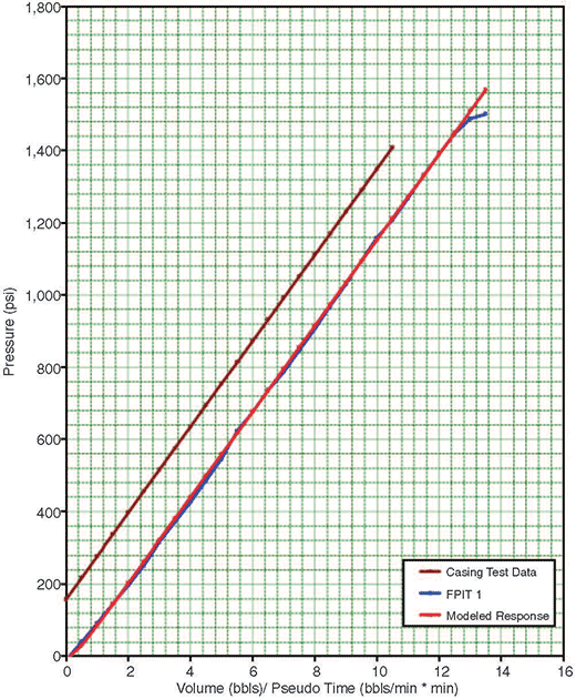
Model of Classic Leak-Off Test

If permeability is not expected to be present in the open hole exposed below the shoe, permeability in the response of the pressure-volume curve suggests a channel may be present that connects permeable formations behind the casing to the test volume. This channel may signal the need for remedial action to seal the channel.

When this occurs, it may be possible to further diagnose the results by spotting a lost circulation pill at the bottom of the well and rerunning the test. If the results display an immediate impact, the permeable formation is likely to be in open hole. If the test shows a delayed response to the pill, permeability is likely behind the shoe and the delay is associated with displacing the pill up the channel to the permeable formation.

FPIT Examples

Figure 4 shows a classic leak-off version of an FPIT in which the test stopped as soon as departure from linearity was recognized. The slope of the test is very close to the slope of the casing test. There is a very slight upward curvature at the very beginning of the test that indicates a small amount of air present. The best fit used 0.55 barrels of air to fit that slight upward curvature. No permeability was required to model the response.

The data were hand-recorded by the well site supervisor in 0.5-barrel increments at a pump rate of 0.5 barrels a minute. The inaccuracies with the hand recording are likely the root cause of the slight waviness of the measured data.

This test was run with synthetic mud. Departure from linearity would be interpreted as being between 1,450 and 1,510 psi. A more accurate determination cannot be made without more finely measured data.

FIGURE 5

Example with Permeability Present

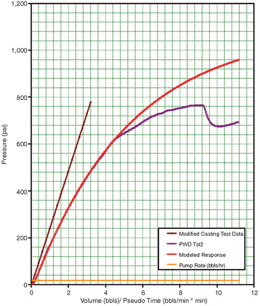
Figure 5 is an example of a test run in the presence of a highly permeable formation exposed at the time of the test. The digital data were taken directly from the annular-pressure-while-drilling (APWD) sensor in the measurement-while-drilling tool, which was down hole a few meters above the shoe at the time of the test. The APWD digital data were merged with the cement unit digital data using time stamps so that the observed pressure from the APWD was tied to the measured pumped volume from the cement unit. The data are sampled in 10-second intervals. The test was run with synthetic mud in the well at a pump rate of 0.3 bbl/minute.

There is no linear characteristic to the pressure-volume curve; it has a downward curvature from the very beginning of the test. The well pressure is greater than the pore pressure before any pressure is applied to the well. Therefore, losses are occurring before the test begins. The calculated loss rate, based on the early time data, is 5.4 barrels an hour. As pressure increased, the loss rate increased because of the higher differential pressure between the bore hole and the formation. When the fracture was initiated, the loss rate to permeability climbed to 7.66 bbl/hour.

FIGURE 6

Example with Channel Present

The optimum model fit to the measured data is found using 0.06 barrels of air present and average mobility of 5.23 milliDarcies per centipoise (md/cp) over the 6.7 meters of formation exposed below the shoe. The fracture initiation pressure can be identified as the point where the measured data depart from the modeled data, and occurs at 626 psi.

Sequential Leak-Off Tests

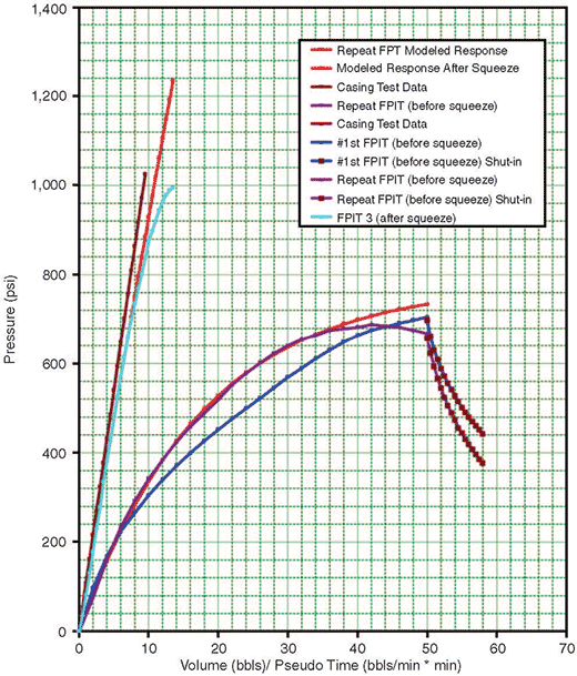
Figure 6 shows a sequence of three leak-off tests run with a water-based mud. The data were hand-recorded by the well site supervisor in 0.5-barrel increments and the pump rate was 0.5 bbl/minute. The first test (blue curve) never reached breakdown pressure. The test was repeated immediately with the same fluid in the well (maroon curve). The model was run (the overlying right-most red curve) and found a good fit between the model buildup behavior and recorded data. Deviation from the model would imply that a fracture was induced at 680 psi surface pressure.

The shoe was squeezed and the test was run a third time. It showed very little permeability present, with much closer conformance to the CIT and a much higher LOP before the fracture was induced.

Attempts to model the first curve were not able to get a good fit. It is believed that was the result of having a different fluid in the channel from that in the well. The model was unable to get a good fit because the formation was exposed to different-viscosity fluids as new fluid displaced the fluids from the cement job. By the time the second test was run, most of the annulus was displaced to drilling mud and a single fluid remained, giving a good fit to the data.

FIGURE 7

Tests with and without LCM

This test has a number of attributes that seem to indicate a channel is present. The first attribute is the large volume of mud required to reach maximum pressure on the first two tests (tests stopped after pumping 50 barrels). After the squeeze, it took only six barrels to achieve the same pressure.

The second attribute is the poor repeatability between the first and second tests, suggesting the permeable formation saw different viscosity fluids pass by while the first test was pumped. The third attribute is the very high permeability required to fit the data.

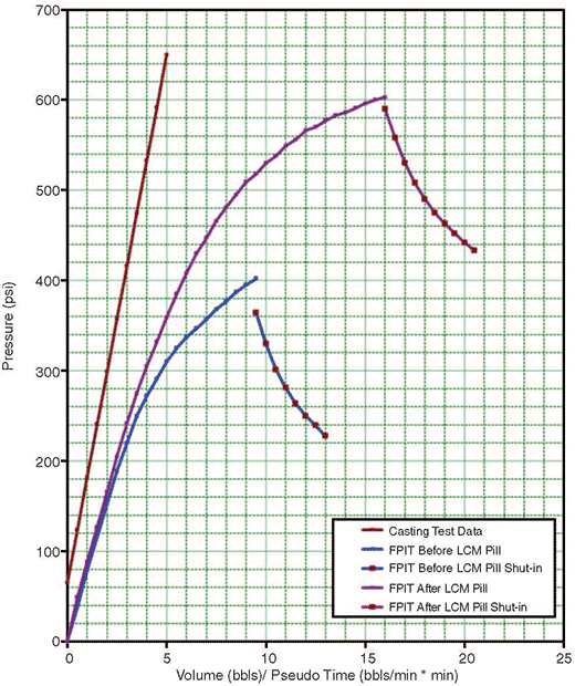
One proactive way to determine whether the permeability is below the casing shoe or is in a channel behind the casing is to run the test initially with the drilling mud in a conventional manner, and then repeat the test with a lost circulation material (LCM) pill spotted in the open hole below the shoe. The LCM should have a contrasting higher viscosity to impact the loss rate into the formation and contain wellbore strengthening material to increase fracture resistance.

If the pressure-volume curve responds immediately to the pill’s presence, permeability is below the shoe. If the response to the pill is delayed, then the pill needed to be displaced up a channel behind the casing to impact losses into sand.

Figure 7 shows a case where this was performed on a well. The blue curve was run with a water-base mud. The data were hand recorded by the well site supervisor in 0.5-barrel increments, and the test was run at 0.5 bbl/minute. The initial test identified the presence of permeability through the characteristic downward curvature. The rig needed to know if a remedial cement job was required to eliminate the possibility of a channel behind the casing.

FIGURE 8

Model Fit to LCM Case

A 50-barrel LCM pill containing 30 pounds per barrel (ppb) of 50-micron D50 calcium carbonate and 20 ppb of 150-micron D50 calcium carbonate was spotted in the open hole, and the second test (the maroon curve) was recorded. The response to the LCM pill was immediate, and the conclusion was made that the exposed permeability was in open hole below the shoe and a remedial cement squeeze was unwarranted.

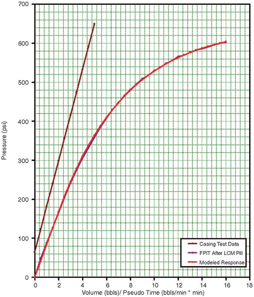
Figure 8 displays the model fit to the second test run with the LCM pill. There is a good fit of the model to the pressure-volume data using no air trapped in lines and 32.5 md/cp over the 2.7 meters of open hole below the shoe. The model results further support the conclusion that the sand is below the shoe in the respect that there is no need to add volume to the system that would occur if a channel was present, and that the value for the permeability required is consistent with expectations for permeable lithologies at this depth and in this area.

Editor’s Note: The preceding article was adapted from IADC/SPE 167945, a technical paper presented at the 2014 International Association of Drilling Contractors/Society of Petroleum Engineers Drilling Conference & Exhibition, held March 4-6 in Fort Worth.