HOUSTON–A few of the most important questions when fracturing tight, unconventional reservoirs are how much the treatment program actually increased the production rate and volume, whether the treatment skipped over significant portions of pay (thereby causing lost revenue), and whether it “double dipped” into pay (thereby wasting significant capital on a redundant completion effort).

Wouldn’t it be helpful to be a “fly on the wall” and be able to peek into the subsurface and watch what is happening where the rocks are being broken? The industry does not have that capability yet, but operators do have some old and new tools. When combined, these technologies can enable data to be time-lapsed in a “movie-like” depiction of subsurface fracturing operations.

The mix of today’s real-time and post-hydraulic-fracture analytical methods includes microseismic monitoring, tilt meter mapping, recording real-time fluctuations in stimulation fluid and proppant rates and pressures, radioactive tracers, and production logs. Another concept may prove useful in creating a way to peer into the subsurface to view fractures opening and closing: using repeated, rapid-time-lapse vertical seismic profiling (VSP) measurements during and shortly after treatment.

The notion is that while the fracture is open and filled with fluid, it forms a good shear-wave reflector (or diffractor), which provides the ability to watch hydraulic fractures open during treatment in a time-lapse fashion. After pumping has stopped and the fluid pressure drops, the fracture face closes on any proppant it contains, causing it to stiffen and lose its ability to reflect (diffract) shear waves.

FIGURE 1

Profile View of Lost Hills Acquisition Geometry (Left) And Time-Lapse Waveforms for Stages 2 and 3 (Right)

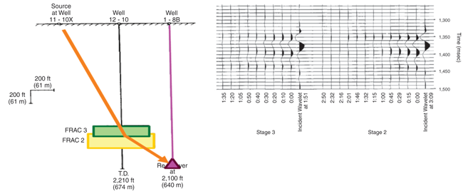
Source: Modified from Meadows and Winterstein (1994)

Field Experiments

As part of a field experiment conducted in the Lost Hills Field in California in the 1990s, Chevron collected a time-lapse S-wave data set after each stage of a hydraulic fracture. The left side of Figure 1 shows a profile view of the acquisition geometry where a surface S-wave source was located near well 11-10X. Two stages of hydraulic fracturing in well 12-10 were monitored successfully using a three-component geophone (pink triangle) near the bottom of Well 1-8B. 

During the period shortly after each stage was completed, when the pumps had been turned off, the shear-wave source was energized every 15 minutes for up to three hours. The S-wave data recorded in the well were rotated so that the XX component was oriented with source and receiver particle motions perpendicular to the direction of the expected fracture plane. The time-lapse traces of the XX component for the third and second stages are shown on the right side of Figure 1.

The elapsed time in hours and minutes since pumping stopped is labeled on the horizontal axis, increasing from right to left. The time down each trace in milliseconds is shown vertically. The right-most trace in each panel shows the incident wavelet, which was approximated by the last trace recorded for that fracture stage. The incident wavelet was subtracted from each of the corresponding recorded traces, yielding the set of time-lapse traces shown.

Immediately after the pumps shut off, there was a large diffracted event, whose amplitude appears to be about 30 percent or more of the incident wavelet. Because the diffracted wavelet is very similar to the incident wavelet, it is unlikely that the origin of this event is from fracture-induced attenuation or velocity anisotropy. It appears to be a separate event, which has diffracted off the fracture plane. The amplitude of this diffracted event drops every time it is measured until it is fairly small at about one hour in elapsed time.

The interpretation was that as the fluid pressure leaked off, the fracture faces came back together and stiffened, no longer acting as a shear-wave diffractor. Even with proppant in the fracture plane, it was surmised that the fracture plane was no longer very compliant and was essentially invisible to S-waves.

The beauty of this experiment was that by using a shear-wave source, energized multiple times over an hour or two after treatment had stopped, a series of measurements was made that showed a diffracted S-wave event coming off the fracture plane. Time-lapse studies are always subject to noise. If only two measurements had been made, any noise in the data would show up as a potential difference. But by making a series of time-lapse measurements, random noise was not a factor and the systematic closing of the fracture was documented clearly.

Encana collected a time-lapse data set using a P-wave vibrator source before and after hydraulically fracturing five wells in the Jonah Field. The time between the two surveys was about a month. An extensive 3-D VSP data set was acquired using 338 surface shots and 140 bore hole receiver depth levels. The left side of Figure 2 shows three of the treatment well locations (A, B and C) in orange circles, with the microseismic events color-coded for each treatment well.

The VSP data were preprocessed to match in amplitudes and the time-lapse differences were created. The data were then migrated to form the image plane, shown in the right side of Figure 2, connecting the monitor well and treatment well A. Plotted over this image are the microseismic events for well A from the map on the left side of the figure projected onto the image plane. Also plotted on the figure in pink are the intervals where the formation was stimulated. An interesting correlation between the microseismic events and time-lapse image can be seen.

FIGURE 2

Microseismic Event Locations from Five Stimulated Jonah Field Vertical Wells (Left)
And Microseismic Events Plotted over Migrated Time-Lapse VSP Data (Right)

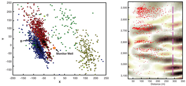
While it may not be exactly transferable from the work at Lost Hills, we expect the fluid-filled fractures lost their high pressure and collapsed around the proppant within a short period after the pumps were turned off. So a time difference of a month between the surveys would have eliminated this effect. However, the effect on the P-waves has not been documented in such a systematic fashion. Therefore, the image in Figure 2 may be caused by several factors, including induced local changes in velocity and attenuation as well as the diffraction of P-waves off the fracture planes. 

Time-Lapse VSP

The proposed new method combines the rapid, time-lapse shear sources at Lost Hills with the time-lapse imaging work done on the Jonah data sets. The acquisition and processing steps include:

• Deploying a microseismic monitoring system with multiple fixed levels of three-component geophones in a single well or multiple wells near the fracture treatment well;

• Continuously monitoring for microseismic events during each of the fracturing treatment stages;

• Deploying an S-wave source to a select set of surface locations;

• Energizing the S-wave source at the selected locations during and after each fracture stage about every 15 minutes and recording the VSP data with microseismic geophones;

• Preprocessing the recorded VSP S-wave data to enhance the shear energy;

• Creating time-lapse traces by subtracting the first (prefrac) trace or the last (post-frac) trace from each trace recorded in each stage;

• Selecting an imaging plane through the center of the microseismic cloud of events for each stage;

• Migrating the time-lapse traces into the imaging plane, creating one movie-like image frame for every 15 minutes during the fracture treatment; and

• Analyzing the movie of images to locate the fluid-filled portions of the fracture.

This method could be used as an add-on to microseismic monitoring. As such, it is only a small additional cost to collect time-lapse VSP data using the microseismic geophone string. Using a small number of spatially distributed surface sources will allow enough fold coverage for a migrated image to be created of the fracture plane without requiring a lot of field time to acquire the shots.

Because of the small number of shots, the acquisition will be set up to be mostly 2-D, and therefore, will lack full 3-D illumination. However, by using microseismic events to define the imaging plane where the fractures have formed, the image can be placed close to its proper 3-D location using “side swipe,” out-of-plane diffracted energy.

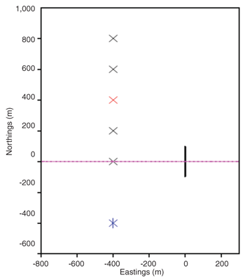
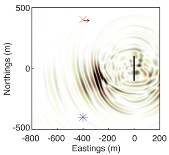
Figure 3 shows the map view of one possible acquisition geometry to collect rapid, time-lapse VSP data. The monitor well is shown by the blue star and the “Xs” denote the set of surface S-wave sources. The fracture is shown by the vertical black line and the horizontal treatment well is the pink line. The idea is to deploy enough shots to illuminate the fracture plane and allow its spatial delineation. Many source-point locations distributed in a 3-D pattern would be ideal, but the time it would take to shoot the pattern would be too long and disruptive to microseismic monitoring. So a limited number of, say, five shots can be selected, most likely along a 2-D line.

FIGURE 3

Map View of Proposed Acquisition Geometry

Synthetic Marcellus Data

To demonstrate this method, a set of synthetic S-wave VSP data was created for the acquisition geometry in Figure 3 using an elastic velocity model fashioned after the Marcellus Shale in Bradford County, Pa., with 64 horizontal layers. The blocked P-wave (blue) and S-wave (red) velocity logs are shown in the left panel of Figure 4. A set of VSP traces for the five shots shown in Figure 3 were generated for a model without a fracture and another one with a single discrete, vertical fracture plane. The fracture plane (44 meters tall and 200 meters long) is located in the Upper Marcellus and its upper and lower extent is shown in green in Figure 4.

FIGURE 4

Model Velocity Profile (Left), Example VSP Record (Center) And Time-Lapse Difference Record (Right)

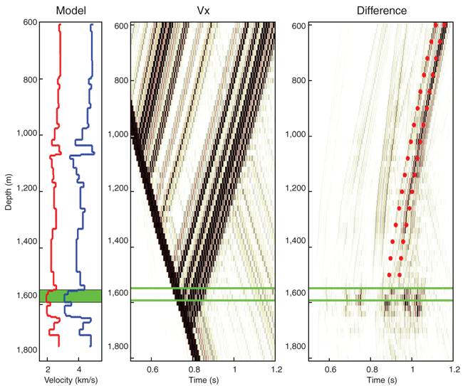
One of the VSP records for the shot located at 400 meters north (red X in Figure 3) is shown in the middle panel of Figure 4. This model contained the single fracture. The panel to the right shows the difference between the model with and without the fracture. The red dots denote the approximate predicted arrival times of the diffracted S-waves from the fracture plane.

These waves propagated as SS waves (shear waves from the source) and were diffracted as shear waves to the receivers. Earlier events on this record can be seen, which propagated as SP (S-wave to the fracture and P-wave to the receivers), PS (P-wave to the fracture and S-wave to the receivers), and PP (P-wave to the fracture and P-wave to the receivers).

To help visualize the diffracted waves coming off the fracture plane, Figure 5 shows a snapshot of the time-lapse wave field at a depth of 1,500 meters (which is above the reservoir) and at a time of 0.84 seconds. The fracture plane is shown by the black line, the source location by the red X, and the monitor well by the blue star. This type of measurement is not possible to collect in the field because it would require a dense spatial network of buried geophones near the depth of the reservoir. However, because this is model data, it is possible to capture this information during the numerical finite difference modeling work.

FIGURE 5

Snapshot of Time-Lapse Wave Field

The diffracted wave field is complicated with several expanding wave fronts. Fortunately, the largest amplitude event is the SS wave, which is used for imaging the fracture plane. It is also clear that there is an amplitude radiation pattern imposed on it, with the largest amplitude heading west-southwest at 20 degrees from due west.

The final two steps are to define an imaging plane and migrate the time-lapse data into it. With model data, the exact position of the fracture plane is known completely. This would not be the case for field data, so the microseismic data provide a reasonable estimate of where fracturing is occurring and define the image plane. Since the frequency content of microseismic data (about 200 hertz) is much higher than VSP data (about 40 hertz), the exact position of the imaging plane is not as important, since the final image will not have as much potential resolution as the locations of microseismic events. 

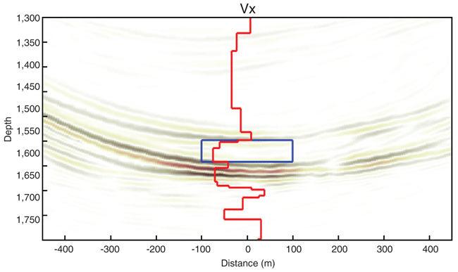
The migrated image constructed along the direction of the fracture plane using the five shear wave shots is shown in Figure 6. The time-lapse traces, with particle motion oriented east-to-west, were migrated with the model S-wave velocity. The blue box shows the exact position of the fracture plane. The red line shows the S-wave velocity log for reference. The image shows that the top and bottom of the fracture plane are well defined with migration sweeps trending upward at the edges.

For this image, only receivers above the reservoir were used in the migration. This is because it is frequently the case that a producing well is used as a monitor well. When this is done, a bridge plug is placed above the reservoir zone, restricting bore hole geophone positioning to above the plug. Most of the energy is sent downward for diffracted P-waves off a single fracture plane. If this also holds true for S-waves, we would expect that the energy measured in the S-wave VSP would be from downward-going diffracted shear waves that reflected upward from strong velocity impedance contrasts below the reservoir.

FIGURE 6

Migrated Image of Time-Lapse Traces from Five Shots in Figure 3

If this is indeed the case, an improved image of the fracture system may be achieved using a reverse-time depth migration algorithm rather than the Kirchhoff algorithm. This is because a reverse-time migration algorithm is intrinsically set up to image using multiple reflections, while a Kirchhoff migration typically uses only primary reflections.

Creating A Movie

Images created with this new method promise to detect areas in the reservoir with fluid-filled fractures. Based on the Lost Hills experiment, the fluid-filled fracture will diffract shear waves, allowing it to be imaged. By inference, if the fluid is not filling the fracture plane, it will be invisible to S-waves and not recorded on the migrated image. Capturing a series of time-lapse images will allow a movie to be created to show fractures opening and closing when the fluid pressure rises and then drops. However, expectations about the spatial resolution of the image must be tempered with the realization that VSP frequencies are a factor of five or more lower than microseismic events.

While microseismic events define a “cloud” of points where rocks break and slip, we are never sure where fluid communication is happening. It may be that at least some of these microseismic events are not associated with useful, fluid-conductive fractures. Combining the seemingly “higher-resolution” image of the fracture system from microseismic with “lower-resolution” S-wave VSP images allows a way to estimate those portions of the fracture plane containing fluid during the treatment. Of course, after the pressure drops and the fracture stiffens, shear-wave VSP image will no longer see the fracture itself.

On a more practical side, acquisition model studies can be conducted ahead of time to determine the optimal number and positions of S-wave sources. If more source locations are needed to obtain a better image of the fracture plane, then perhaps the time interval between the shots could be increased. Also, the required number and positions of bore hole geophones should be determined.

All these factors must be taken into account to make this an economically successful method to peer into the reservoir and observe fractures in a way that helps answer questions about whether a treatment was successful at tapping the entire reservoir without overstimulating.

Editor’s Note: The author acknowledges the Society of Exploration Geophysicists for permission to publish some of the information in the preceding article. Data on the Lost Hills Field was presented in a paper authored by M. A. Meadows and D. F. Winterstein and published in Geophysics, Vol. 51, 1994 (“Seismic Detection of a Hydraulic Fracture Shear-Wave VSP Data at Lost Hills Field”). Data on the Jonah Field project were adapted from technical papers at SEG’s 79th Annual Meeting (“Fracture Quality Images from 4-D VSP and Microseismic Data at Jonah Field,” by M. E. Willis, D.R. Burns, J. Shemeta and N.J. House) and the European Association of Geoscientists & Engineers’ 74th Conference & Exhibition (“Advancing the Use of Rapid Time-Lapse Shear-Wave VSPs for Capturing Diffractions from Hydraulic Fractures to Estimate Fracture Dimensions,” by M. E. Willis, X. Fang, D. Pei, X. Shang and C.H. Cheng).