Microseismic data acquired at the Hydraulic Fracturing Test Site 2 (HFTS2) in the Delaware Basin suggests that hydraulic fracturing fluids tend to find the weakest passages through geologic formations. The data also indicates relative well positions and treatment sequence significantly impact fracture geometry.

The microseismic data was collected as part of a program aimed at supporting continued advances in hydraulic fracturing efficiency, which already have helped make the Wolfcamp the largest continuous oil and gas formation in the United States. The data was acquired during the completions of three Wolfcamp wells–the Boxwood 1H, 2H and 4H–that were stimulated sequentially.

When the Boxwood 1H was stimulated, its toe stages quickly reacted to the depleted Bitterroot section to the east of the Boxwood pad, extending microseismic events more than 3,000 feet eastward. This behavior changed dramatically after the treatment passed the Bitterroot section at the toe; the heel stages showed tight microseismic grouping around the stimulated well, a sign treatment was breaking up virgin reservoir rock.

The Boxwood 2H demonstrated a similar pattern of behavior between its toe and heel stages, suggesting the depleted Bitterroot remained easier to refracture than adjacent nondepleted rock.

However, microseismic activity differed for the Boxwood 4H treatment. The events generated during the 4H’s stimulation were hardly influenced by the depleted Bitterroot and filled the space between the previously stimulated 1H and 2H wells.

These observations come from advanced microseismic monitoring techniques, including:

• Native synchronization of five monitor arrays;
• Real-time location of microseismic events;
• Joint event-hypocenter/velocity-model inversion that locates microseismic events while simultaneously constructing azimuthally anisotropic velocity models; and
• High-resolution reservoir imaging, utilizing microseismic events as downhole sources.

Acquisition Geometry

To ensure microseismic interpretation would remain consistent across the three wells, a geometry with five static monitoring arrays was established to acquire and process the data. Beginning in March 2019, three individual completions of one-mile laterals drilled in the Wolfcamp and Wolfcamp B were monitored with this arrangement. The arrays were static throughout the entire operation, except for a redeployment at 2H stage 5 landing at the same position in the Boxwood 55-1-12 Unit 5PH. All arrays were sampled at a rate of one sample every 0.25 milliseconds.

The 40-level vertical array in the Boxwood 55-1-12 Unit 5PH was deployed with 50-foot receiver spacing totaling 2,000 feet of array extension. Two horizontal arrays in the Boxwood 55-1-12 Unit 3H were deployed as a single split-whip array with 100-foot receiver spacing to the toe. The horizontal arrays had 1,300 and 1,400 feet of length, respectively, and were separated by a 1,500-foot interconnect cable.

For Thresher 55-1-12 Unit A 16H, a single split-whip array with 100-foot spacing was deployed to straddle the well’s heel, with one array in the horizontal section and the other in the vertical section. The vertical and horizontal arrays had 1,300 feet and 1,400 feet of length, respectively, separated by 1,500 feet of interconnected cable. The standard Geospace DS150 geophones had magnetic coupling in the vertical sections and gravity coupling with no magnetic components for the horizontal arrays.

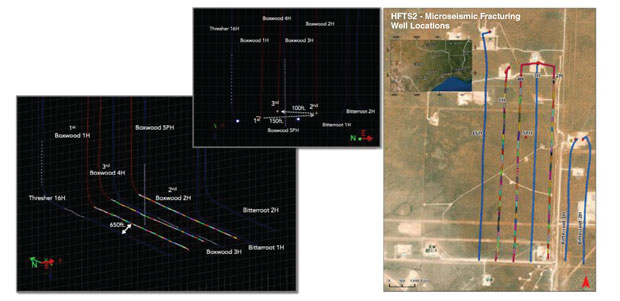
Figure 1 illustrates the position of the treatment and monitor wells. On the first (toe) half of acquisition, events were detected primarily on the Boxwood 55-1-12 3H’s horizontal arrays. As the completion progressed, events easily were detected by the Boxwood 55-1-12 5PH array. Events in the heel-half were detected by Thresher 55-1-12 Unit A 16H arrays as the completions moved toward the heels.

FIGURE 1

Well Geometrics and Locations

All data was natively synchronized on a single recording system, including all channels on all arrays. In other words, every single channel for all the receivers in all the monitor wells was connected to and recorded by a single acquisition system, as if they were a single array, and merged into a single trace gather in the processing phase. This specific setup is critical because the native sample is not recoverable if each array is recorded independently and merged. The approach eliminates the possibility of synchronization uncertainty.

Processing

Clearly identifiable P- and S-wave arrivals must be evident from a given array to be incorporated into processing and locating that event. For this reason, data from the array most distant from an event usually was excluded from multiarray event location. This meant that events associated with the toe-half stages excluded data from the Thresher 55-1-12 Unit A 16H array. Similarly, horizontal arrays in the Boxwood 55-1-12 3H were used to process heel-half stages only if the sources generated clearly identifiable P- and S-wave arrivals.

Triggering is the first step in the proprietary processing workflow. It detected microseismic events in the continuously recorded data. By applying image processing techniques, the algorithm automatically classified the continuous data and categorized it based on noise level. Data segments with medium to low noise are likely to contain microseismic events with visible P- and S-waves.

The highest-quality events’ direct P- and S-wave arrival times were used for velocity model building. The key differentiator of our processing is that we built the velocity model based on both perforation shots and microseismic events. The advantage of incorporating microseismic events to constrain the velocity model is that it significantly increases reservoir sampling compared with the traditional method of relying solely on perforation shots.

Events carry velocity model information along their ray paths. By adding them to the velocity model building, sampling of velocity variations in different azimuths and geologic formations is improved, eliminating extrapolation of the observed reservoir character along many different azimuths that could introduce significant event location error.

This allows the construction of a layered azimuthally anisotropic velocity model that fits the travel time data of both perforation shots and events. During post-processing, additional high-quality events are incorporated to further constrain the velocity model, and all the events are reinverted using this final velocity model. To eliminate unknown origin times, only sources with both P- and S-waves picked in at least one vertical and one horizontal array were used.

Second Path

The second way events are located is using joint inversion or tomography and calculating its properties. (High-quality events used for velocity model building also pass through this step.) Many of the events are posted to an online portal during real-time monitoring. Time constraints keep us from going through every trigger file and posting every event in real time, but we look at the remaining files during post-processing to add the missing events.

Additionally, as a quality control process, the picked times of located events are reviewed and events that did not pass the misfit threshold are reprocessed. The misfit is the root-mean-square average of the difference between picked arrival times and model-predicted arrival times. The predicted arrival times are calculated with two-point dynamic ray tracing using the final velocity model.

The HFTS2 project used a threshold of 2.5 milliseconds. Events with misfits above 2.5 milliseconds were reviewed and reprocessed when necessary. If a reprocessed event still fell outside the misfit threshold, it was usually because of misidentified arrivals related to a high level of noise.

Separate toe and heel velocity models were computed for each treatment well. Separate models were built for each well because events at the toe stages set on rock that had yet not been fractured, while the heel stages were in a part where rock was more likely stimulated.

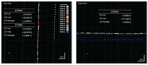
To quality control the velocity model, perforation shots were relocated to compare the model-predicted relocations using the final velocity model with known perforation locations. As shown in Figure 2, those errors can be used to quantify the upper bounds of location error for the microseismic events.

FIGURE 2

Perforation Shot Relocations

Data Imaging

After being located, microseismic events are used as sources to illuminate the subsurface. First, we selected high-quality events that would be used to image a volume of the reservoir that contains the treatment wells. Events with high signal-to-noise ratios were selected to ensure they would not add noise to the migrated volume.

Based on the geometry and spatial distribution of the microseismic events, one volume was created to the south of the Boxwood 55-1-12 Unit 5PH (the “southern volume”) and another volume was created to the north (the “northern volume”). Each volume had a different ray fold in accordance with microseismic event locations. The spatial extent of image volumes was selected to reflect the optimally illuminated region. Both volumes had a grid made of five-foot cubes.

The southern volume was computed using 407 events from Boxwood 4H stages 13-16. Those events were illuminating the subsurface likely stimulated by the Boxwood 1H and Boxwood 2H treatments. The northern volume’s calculation involved 386 events from Boxwood 4H stages 24-26. These events illuminated a region stimulated by not only Boxwood 1H and Boxwood 2H, but also Boxwood 4H stages 21-23.

A 3-D Kirchhoff prestack depth migration was applied to the squared-phase trace data and created volumes for P- and fast S-waves. After further analysis of the frequency content and image quality, the fast S-wave volume was used for interpretations. Because the microseismic sources have a high frequency (50-400 Hz), the microseismic volumes derived from the fast S-waves have a remarkably high spatial resolution of approximately 12 feet.

Next, fractures were extracted from image volumes. The project investigated whether the microseismic volumes displayed the major discontinuities that can be tied with surface seismic and nearby well logs. We identified possible seismic stratigraphic terminations, as well as discontinuities that are likely to be related to fractures. Additionally, we overlayed microseismic events to the volume to correlate them and further investigate the discontinuities.

Microseismic Results

After processing the microseismic data, a representative subset of data containing only the highest-quality events was manually selected. This representative dataset was obtained by applying a series of cutoffs to the entire dataset to filter out events with processing limitations, such as large distances, that could cause the hypocenter to be poorly constrained.

The representative dataset is free of events with poorly constrained locations. This was achieved by only including events detected by at least one vertical and one horizontal array. All events with misfits larger than 2.5 milliseconds were excluded as well.

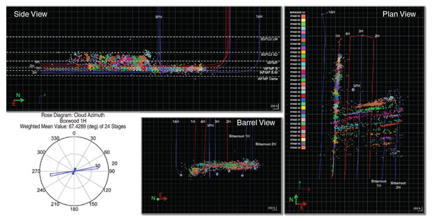
Figure 3 displays the representative events for the Boxwood 1H, the first well to be treated and the farthest from the Bitterroots wells (3,000 feet to the east). Microseismic activity during the treatment of the 1H’s toe-half extends toward the depleted region associated with the Bitterroot wells. Conversely, events from the heel-half stages all are near the treatment well, the pattern seen when stimulating virgin reservoir rock.

FIGURE 3

Representative Microseismic Events For Boxwood 1H

The Boxwood 2H was the next well to be completed and the closest to the depleted region, which was only 1,100 feet eastward. The Boxwood 2H’s fractures preferred to grow eastward toward the Bitterroot wells. However, the heel stages’ stimulation triggered events to the west between the Boxwood 1H and 2H. This reversal in the direction of half-length asymmetry is compelling evidence that, absent a nearby depleted zone, the Boxwood 2H preferentially developed length toward the recently completed Boxwood 1H.

This suggests that microseismic events tend to be triggered on rocks that are easier to refracture because they are in previously fractured zones, rather than virgin reservoir, regardless of the state of depletion. The shallow Wolfcamp formation was the primary conduit for communication from the Boxwood 2H to the Bitterroot wells, and the total event count for the Boxwood 2H was higher than the Boxwood 1H (more distant from the depleted zone). The Boxwood 2H’s treatment also produced more events than the 1H’s.

Boxwood 4H was the last well to be completed, and microseismicity trends from its treatment were distinctly different from its predecessors, as seen in Figure 4. Most of the events associated with the 4H were located between the Boxwood 1H and 2H, regardless of position relative to the Bitterroot wells. This implies pressure walls were created on both sides of the 4H by the stimulations of the 1H and 2H, effectively containing length development.

FIGURE 4

Representative Microseismic Events For Boxwood 4H

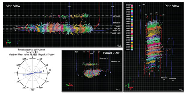
Additionally, low-magnitude microseismic events were recorded in shallow formations at the top of the Bone Springs, indicating this containment encouraged more height growth. Interestingly, an aseismic zone was observed in the middle and bottom sections of the Bone Springs, where few, if any events were triggered. This lack of events was not associated with any geometry limitations, as the hypocenter was well constrained.

Finally, all three Boxwood wells displayed a similar absence of westward length development beyond the Boxwood 1H, toward Thresher 55-1-12 Unit A 16H. Events were restricted to the area of Boxwood 1H, 4H, 2H and Bitterroot 1H and 2H. This indicates that these regions were easier for microseismic event development, since there was no former cause that could prevent hydraulic fracturing from progressing westward.

Imaging Results

Four volumes were created for the microseismic imaging analysis: two derived from P-waves and two from fast S-waves. These volumes exhibit higher resolution and detail than surface seismic volumes. Major reflectors were observed in the microseismic volumes, and these reflectors can be tied with surface seismic and well logs.

Despite differences in microseismic pattern between the heel-half and toe-half stages of the Boxwood wells, the fracture density observed in the northern and southern volumes are similar. This is likely since all events selected as sources for the microseismic volumes were associated with the Boxwood 4H stimulation, which captures the subsurface’s state after the treatment of Boxwood 1H and 2H. The northern volume appears to be more continuous than the southern volume, which has phases being terminated multiple times.

We recognize that microseismic events have grown toward the Bitterroots wells because this region is easier to refracture. It is evidenced by the different imprint from toe and heel stages for Boxwood 1H and 2H, where the heel stages show a more common microseismicity pattern of a virgin reservoir rock treatment.

We also believe the distinct behavior of microseismic events from Boxwood 4H comes from a pressure wall created by the treatments of Boxwood 1H and Boxwood 2H, which forced stimulation to be triggered between those wells.

About the shallow events in the Bone Spring Lime, we infer they occurred because of the pressure wall formed by the stimulation of Boxwood 1H and 2H. Once more fluid is pumped into the subsurface, it increases the pressure of the surroundings and encourages the fracture to grow upward.

A fiber cable was deployed in the Boxwood 55-1-12 Unit 5PH monitor well. Frac hits were detected on it during the treatment of the Boxwood 4H for stages close to the monitor well. This observation agreed with the microseismic results and confirmed our hypothesis.

Editor’s Note: For more detail on this study, including figures showing the microseismic imaging volumes, see “Microseismic at HFTS2: A Story of Three Stimulated Wells,” a paper originally prepared for presentation at the 2021 Unconventional Resource Technology Conference. The study is based on work supported by the Department of Energy under Award Number DE-FE0031577. The authors would like to thank Vladimir Grechka (1962-2021) for his contributions, as well as his generosity, friendship and dedication to teaching and mentoring.