MIDLAND–The industry continues to work toward optimizing horizontal well completion designs to effectively develop the Permian Basin Wolfcamp Shale. Many completion variables directly impact the performance of Wolfcamp horizontal wells, including fracture stages per well, fracture type, average water requirements, proppant type, fluid type, proppant size, average pump rate, hydraulic horsepower per stage, pounds/foot of proppant per stage, number of clusters, cluster spacing and lateral length (completed interval).

Relationships among these variables were studied with the help of advanced multivariate regression (supervised machine learning) techniques, which allow for the group-wise inclusion/exclusion of factor variables. The analysis was performed on 201 horizontals in the Wolfcamp play (A through D benches) with available data. The analysis identified key parameters that could be used to predict the number of fracture stages. Three additional models were introduced to answer the following questions:

• How many clusters per fracture stage?
• How many perforations per cluster?
• What is the spacing between clusters?

This new methodology can predict the number of fracture stages and optimize completion strategies in Wolfcamp wells. The pool of independent (or input) variables considered in the model to predict fracture stages (the dependent variable) include county, depth, reservoir type, overlap between horizontal wells’ drainage volumes, volume of injected fluid per stage, true vertical depth, proppant volumes, gas yield, cumulative oil and cumulative natural gas, estimated ultimate recoveries of both oil and gas, and initial 30-day and 60-day production rates for both oil and gas.

The model relates the 30-day IP of oil to the number of fracture stages for horizontal wells. According to the concept, stages vary by county and reservoir, and also according to 23 distinct completion variables used in developing the model. The parameters ranged from completed feet of lateral to cluster spacing, average proppant concentration, gas-to-oil ratio and initial reservoir pressure.

Optimizing Completion Designs

For years, the industry has employed zipper fracturing, modified zipper fracturing and sequential fracturing approaches for stimulating unconventional reservoirs. These placement methods activate more natural fractures and may increase production from shale reservoirs. On the other hand, some operators prefer the engineering design of fracture stage placement based on equal spacing. With any of these approaches, multivariate regression can analyze the relationships among variables.

The number of fracture stages has increased with time in all shale gas and tight oil plays along with increases in the proppant and fluid volumes, lateral lengths, and fluid injected and proppant pumped per foot of lateral. In fact, proppant volume per foot in horizontal wells has increased 500% during the past eight years, fluids have increased 800%, and average lateral lengths have doubled. The 12-month cumulative production per 4,500 feet of lateral doubled during the same period.

The industry’s Wolfcamp completion designs continue to optimize each of these variables. The number of fracture stages is a key aspect of the completion design that impacts other variables, such as proppant and fluid volumes. The workflow involves two main stages.

The first stage is to develop a user-friendly model to predict fracture stages using a multivariate linear regression for the four outputs (stages, perforations, clusters and spacing) to fit the data using the “group lasso” method. This relatively new approach was devised for multitask machine learning applications, where strong correlation exists among the outputs, while also incorporating shrinkage and model selection.

The second stage entails testing the model using in-sample test data and publicly available information. While the global model was fitted to the four outputs, this article focuses only on the results of the model for frac stages.

Predictive Model

The model shows relatively good in-sample predictions, as shown in Figure 1, which displays the actual observed values of outputs on the y-axis versus their model-predicted values on the x-axis. The model multiplies the model coefficients (B values) with their corresponding inputs to produce the output.

FIGURE 1

Predicted versus Actual Number of Stages

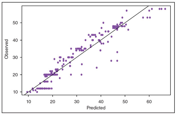
FIGURE 2

Pairs Plot of Stages by County and Reservoir
(Colored According to Reservoir)

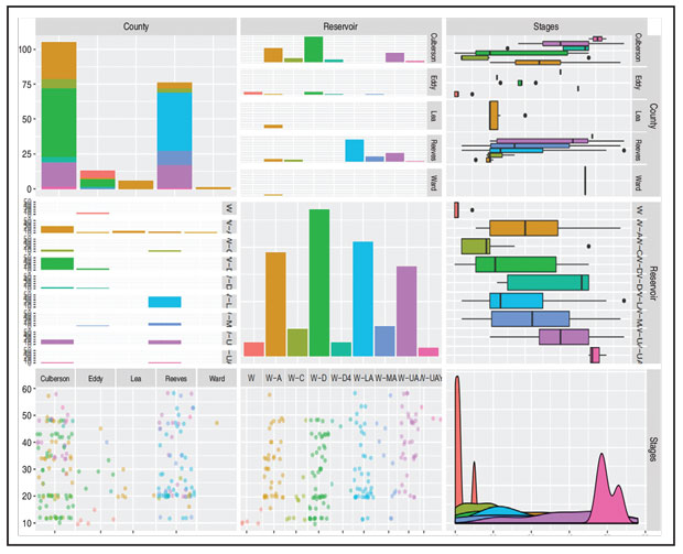
Figure 2 shows a pairs plot of stages by county and reservoir (colored according to reservoir). From the clear separation of colors on the bottom right-most panel (representing the distribution of stages), it is immediately apparent that reservoir (and to a lesser extent county) is a very good predictor of stages.

The strong correlation among the four outputs makes it challenging to apply standard multivariate linear regression models (multitask machine learning). This, and the fact that almost half the input parameters are group variables (categorical inputs), suggests a predictive model with the flexibility of incorporating sparsity (or shrinkage of model coefficients) may be warranted. Therefore, the decision was made to incorporate the group lasso model, whereby the coefficients in each of the two groups of categorical inputs are shrunk together. In the final model, county and reservoir were found to be the most important predictors.

An analysis of the goodness-of-fit of the model can be seen in Figure 1, which compares the actual versus model-predicted values of stages. However, the usefulness of this in-sample analysis is limited because it does not reveal much about the model’s predictive ability on out-of-sample data.

Machine-Learning Procedures

One of the standard machine-learning procedures to validate a selected model on out-of-sample data is to carry out a K-fold cross-validation (KCV) exercise. This step was performed for the chosen model using K=5. Consequently, in each test/training set split of the data, four-fifths of the data was used to fit a group lasso model and generate predicted values for the remaining fifth. The percent absolute relative prediction error (ARPE) was used to assess prediction quality.

FIGURE 3

Percentage of Absolute Relative Prediction Errors

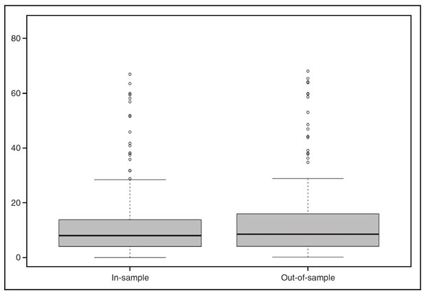
The results appear in Figure 3, the right panel of which displays box plots of the in-sample and out-of-sample ARPE values. Note that for the in-sample ARPEs, KCV is not carried out (i.e., the model is fitted to the entire dataset and then used to generate predictions for each of the 201 Wolfcamp wells). Naturally, we would expect in-sample predictions to fare better, which is indeed the case, with a mean ARPE of 11.9%, compared with 12.9% for out-of-sample.

Lessons learned from completing Wolfcamp wells in the Permian Basin will guide future best practices. Technology certainly has a role to play, as demonstrated by the new model to predict the number of frac stages. Using outputs of actual data from Wolfcamp wells to guide input selection, the approach gives operators a new tool for quickly estimating the number of fracture stages per well. The model proved accurate when tested on publicly available Wolfcamp well data. As a final recommendation, additional models could be proposed in future work with the collection of additional data, and intensive selection may begin on Wolfcamp completion designs in the Delaware Basin.

Editor’s Note: The authors acknowledge Cimarex Energy for providing the data used in this work.