Frac Design

HOUSTON–Determining the appropriate spacing of hydraulic fracturing stages is an important step in optimizing the performance of horizontal wells with multistage completions in unconventional resource plays.

While the general trend across the industry has been toward higher stage counts and tighter stage spacing, experience shows production performance does not scale up in simple increments when fracture stages are added in closely spaced completions. In fact, instead of adding hydrocarbon production on a per-stage basis, tighter spacing can add incrementally less hydrocarbon production per stage.

To determine the most effective stage spacing, Hess Corporation is deploying downhole geophones in Bakken and Utica shale wells to monitor microseismic events associated with multistage hydraulic fracturing at different stage intervals. The objective is to integrate microseismic and other measurements to optimize the cost-to-benefit ratio of stage spacing without having to drill a large number of wells to assess the impact of frac design changes and geological variables.

Small, 3-D structural models are constructed around each well to create depth histograms of microseismic events measured in relation to a common stratigraphic boundary to assess how hydraulic fractures interact. Stage-to-stage analysis of the histograms shows a systematic interference phenomenon called ‘‘stress shadowing,’’ which causes closely spaced stages to interfere with one another, and to bounce cyclically in and out of zone during multistage fracturing.

Given these observations, Hess has developed a conceptual stress shadowing model for both single and multiple frac stages. Two-dimensional fast Fourier transform (FFT), coefficient correlation, and quantile analyses applied to the histograms identify in-situ stress changes induced by the formation of closely spaced fractures and how those changes influence the propagation of subsequent fractures.

Impact Of Stress Shadowing

Microseismic data measured during multistage hydraulic fracturing of Hess wells indicate stress shadowing exhibits a 3-D behavior. To properly simulate the propagation of multiple fractures for a completion stage in a horizontal well, fracture models need to take into account the interaction between adjacent hydraulic fractures. We plan to apply 3-D stress shadowing theory to our future completion models to optimize stage spacing.

FIGURE 1

Schematic Representation of Stress Shadowing in Lateral With Closely Spaced Hydraulic Fractures (Utica Well A)

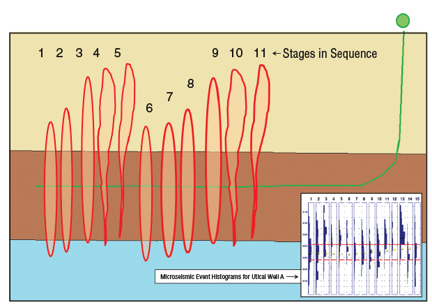
Our concept of stress shadowing’s impact on hydraulic fractures is represented schematically in Figure 1, based on microseismic analysis of a horizontal Utica Shale well. As closely spaced hydraulic fractures develop and interact during a frac stage, stress begins accumulating in the target zone. The stress shadow created increases the minimum horizontal stress in the zone, thereby gradually reducing the stress contrast with the natural barriers that contain the fractures.

As in-zone stress increases, additional fractures will grow preferentially upward and out of zone into the overburden interval (or downward in cases with low underburden stress contrast). As subsequent stages develop and stress accumulates in the area above (or below) the reservoir, fractures begin to reform in the target zone.

Following this pattern, in-zone and out-of-zone fracturing occurs in a repetitive cycle throughout the multistage fracturing process in response to localized stress changes along the lateral. This leads to cyclical variations in frac height for different stages along the wellbore, and predictable variations in productivity should be expected, based on the amount of stress-related frac height growth.

FIGURE 2A

Bakken Production per Well versus Stage Count
(After 30, 90, 180 and 365 Days)

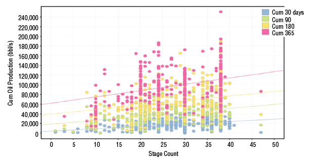
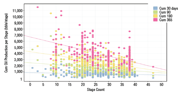
FIGURE 2B

Bakken Production per Stage versus Stage Count (After 30, 90, 180 and 365 Days)

_{Sources: Data from the North Dakota Industrial Commission’s public database; graphs courtesy of Hess Corporation’s Bakken team​}

Figures 2A and 2B show per-well and per-stage production versus stage count, respectively, after 30, 90, 180 and 365 days for Bakken wells. The diminished per-stage returns of closer spacing are evident from the start of production, and likely are the result of the stress interaction between a growing hydraulic fracture and the previous fractures placed in a lateral. We believe the physics controlling incremental per-stage production is related to the observed cyclical reduction of the in-zone fracture area.

Case Study Wells

Case study data from three Hess-operated horizontal wells–two in the Utica play in Ohio and one in the Middle Bakken in the Williston Basin–illustrate the results of analyzing microseismic events to optimize stage spacing and the influence of stress shadowing on closely spaced fractures in multistage completions.

Well A (referenced in Figure 1) is in the Utica and has a 5,000-foot lateral section with 15 stages placed in a plug-and-perf fashion in a cased and cemented borehole. Each stage was 290 feet long with four perforation clusters spaced at 70 feet and about 70 feet from the closest perfs in the previous stage. Well B also is a Utica well with a 5,000-foot lateral. It was cased and cemented with its stages 230 feet apart, each with four perf clusters spaced 50 feet apart. Well C is in the Bakken. It was completed with a hybrid design of 19 sliding-sleeve stages followed by another 10 plug-and-perf stages, all using tubing held in the open hole by packers that pressure isolated the successive stages. It had a 10,000-foot lateral with nominal stage spacing of 250 feet.

In each case, nearby monitor wells were instrumented with geophones to record microseismic events and determine hypocenter locations while the completions took place. Analyzing depth histograms of points grouped by stage provides a statistically significant measure of the depth range encountered by the fracturing process. By creating histograms of the position of microseismic events relative to a prominent stratigraphic boundary, the analysis avoids the confusion that results from the effects of dip over the length of the lateral, or from variations in the placement of the perforated interval where the lateral crosses bedding.

This requires building a 3-D structural model using geosteering results from drilling the lateral to develop a cross-section along the borehole and tops from the monitor well or nearby wells to determine structure away from the lateral. Geosteering provides a one-dimensional view extrapolated into two dimensions along the plane of the lateral, so it does not include variations in layer thickness. However, in these examples, our understanding of the structure is that it is mostly simple, with planar dip in the regions around the wells. A small 8- to 10-foot fault is identified from geosteering in the second stage of well C, with another possible fault in stage 18.

FIGURE 3A

Hypocenter Locations in 3-D Depth View

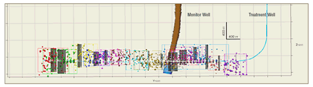
FIGURE 3B

3-D Structural Model Constructed From 2-D Geosteering Profile

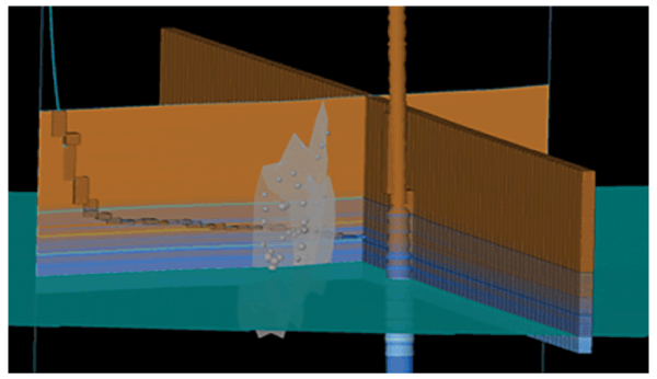
FIGURE 3C

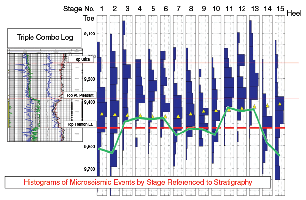
Calculated Depth Histograms of Hypocenter Frequencies Relative Trenton Limestone (Utica Well A)

Depth Histograms

Figures 3A-3C illustrate the process of constructing microseismic event depth histograms for well A in the Utica. Figure 3A shows a profile view of the microseismic hypocenter locations in 3-D depth view relative to the borehole. Figure 3B shows the geosteering profile and 3-D structure near the borehole, with nearby well tops and one stage of events in the gray cloud.

Figure 3C shows calculated histograms of relative frequency of points by depth above the Trenton Limestone (red line) for each stage (the Trenton formation is a prominent carbonate platform underlying the reservoir section). The yellow triangles indicate the average perforation depth for each stage.

On the right side of the plot, the wellbore crosses stratigraphy such that the well lies in the same stratigraphy for stages 1 through 7, and crosses bedding in stages 8 through 15. The green line is the average value of the deepest 15 percent of microseismic events in each stage, representing the quantile at the low side of each histogram.

The results show a clear pattern of two “bounces” of the histogram centers along the length of the borehole capable of significantly impacting the amount of fracture contact within the producing interval. The bounces are evident in the quantile measurement (green line) at the average depth of the deepest 15 percent of microseismic events.

Beginning with the first stage at the toe of the well (left side of the plot), fractures are centered at the borehole. The fractures in the following stages gradually moved upward about 200 feet (stages 3 through 6). They subsequently returned to the borehole in the middle of the well (stages 7 through 10), and the pattern repeated.

Analyzing the histograms with 2-D FFT and correlation coefficients between histograms verified that the microseismic-observed depth histograms behaved in a two-bounce cycle along the well’s axial direction. Each histogram, taken as a series of values representing the relative frequency of points in each depth bin, was correlated with all other histograms. The histograms are similar to their immediate neighbors and to other histograms located six to seven stages distant, and again to histograms located 12-14 stages away (see SPE paper 170924).

FIGURE 4

Normalized ISIP, Maximum Treating Pressure and Job Size (Utica Well A)

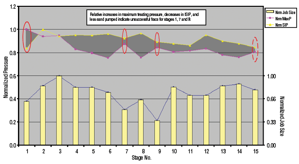
Figure 4 shows normalized instantaneous shut-in pressures (ISIPs) (yellow line), normalized maximum treatment pressure (pink line), and normalized job size index using a product of sand and water pumped (yellow bars) from well A. Comparing these data to Figure 2C, the observed out-of-zone bounces coincide with systematic changes in ISIPs and maximum pressure, as well as difficulty in placing the entire job (indicated by shorter yellow bars).

The lower ISIPs occurred when smaller jobs were not able to develop the same in-zone net pressure or fracture widths. The shorter jobs for stages 1, 7 and 9 coincide with fractures that remained in zone. Stages that bounced upward had bigger job sizes because they were easier to pump. By the time the second bounce returned to the wellbore (stage 15), the engineers already had adjusted by pumping higher-viscosity fluids, which may have helped finish the job.

Tracking Stress Shadowing

Quantile analysis measures the depth of a portion of the histogram. For values that change slowly from one stage to the next, it is a reasonable way to track bounces. Faulting and pump pressures may affect the top of the histogram depth range in any given stage. Following the bottom of the histogram seems best for tracking cycles related to stress shadowing.

The green line in Figure 3C (representing the average value of the deepest 15 percent of points from each histogram) has a loopy, two-bounce structure within the length of the lateral. The stresses were building in the zone of interest as initial stages were pumped, so that at some point, the stresses accumulating in the reservoir zone diminished the stress contrast at the top of the fractures, allowing them to propagate upward. As stress accumulated higher in the section, new fractures were able to reform close to the borehole, and the process repeated.

FIGURE 5A

Induced Stresses Along Fracture Cross-Section (Fracture Height = 300 feet)

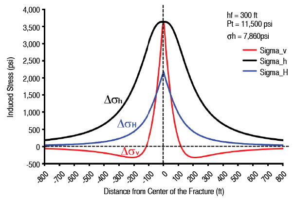
FIGURE 5B

Induced Stresses Along Fracture Cross-Section (Fracture Height = 100 feet)

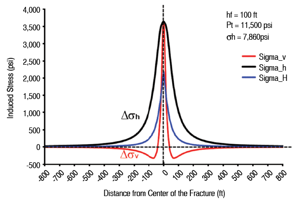
As shown in Figures 5A and 5B, using hydraulic fracturing data from the Bakken formation, the induced, incremental minimum horizontal stress increases as fracture height and injection pressure increase. In this case, treatment pressure was 11,500 psi and in-situ minimum horizontal stress (σ_h) was 7,860 psi, for a net pressure of 3,640 psi. The figures plot the relationship of the induced stresses versus the distance away from the center of a fracture at fracture heights of 300 and 100 feet, respectively.

The treatment pressure exerts a compressive stress in the direction normal to the fracture on top of the minimum in-situ stress that is equal to the net pressure at the fracture face, but quickly falls with distance from the fracture. At a distance beyond one fracture height, the induced stress is only a small fraction of the net pressure.

The stress shadow describes the increase of stress in the direct vicinity of this fracture. If a second hydraulic fracture is created parallel to the existing open fracture within the stress shadow, it will have a closure stress greater than the original in-situ stress, requiring a higher fracture initiation pressure.

This modeling indicates that a typical hydraulic fracture with a height of 300 feet (Figure 5A) causes a significant increase in the minimum horizontal stresses for distances less than 300 feet from the fracture. This implies that if the spacing of the two hydraulic fractures is less than 300 feet, strong stress shadowing should be expected.

Our observations show that a greater fracture height has a larger impact area of the stress, and that smaller hydraulic fracture spacing creates a stronger stress shadow and stress impact. In fact, the induced stresses may change the in-situ stress state, stress direction, and stress regimes in the interference area, causing subsequent fractures to grow in an irregular fashion.

Minimum Horizontal Stress

Fracture initiation pressure (p_b) is much more dependent on minimum horizontal stress than the other in-situ stresses. If a change in minimum horizontal stress is large enough, it will alter the fracture initiation position and propagation direction. Our observations indicate stress shadowing increases minimum horizontal stress, increases p_b, and makes the formation harder to fracture.

When the stress increase is significant, particularly in the case of closely spaced hydraulic fractures, it will cause new hydraulic fractures to redirect. This often results in fracture growth and propagation preferentially upward, if the minimum horizontal stress is lower in the shallower formation.

FIGURE 6

Conceptual Model of Changes in Minimum Horizontal Stress Resulting from Closely Spaced Fractures (Bakken Well)

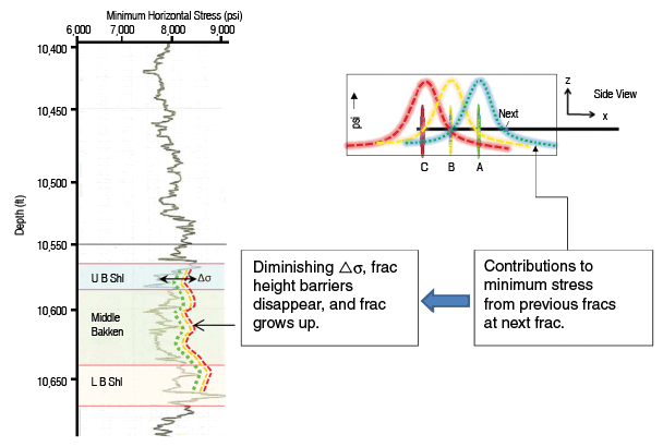
Figure 6 shows the original in-situ stress estimated from logs in a vertical Bakken well. The right side of the figure illustrates how stress shadowing increased the minimum horizontal stress after three parallel fractures were generated. The dashed lines show the sequentially elevated minimum stress (stress shadow) as fractures were added.

After three fractures were generated, the minimum stress at the location of the fourth frac was highly altered, and the stress barrier above the reservoir almost disappeared as the stress shadow increased the minimum horizontal stress in the planned fracture zone, and reduced the stress contrast with the overburden. The result was that subsequent hydraulic fractures grew upward because of the reduced stress contrast between the target reservoir and the overburden.

‘Self-Correcting’ Process

Figures 7 and 8 show the histogram results from well B (Utica) and well C (Bakken), verifying the observations in well A. The 19-stage well B (Figure 7) has 230 feet of spacing between stages (compared with 290 feet in well A), and more sand was pumped than in well A. The well showed three or four bounces, with a characteristic spacing of 1,320 feet per bounce. The red line denotes the top of the Trenton Limestone, and the green line is the quantile contour at the top of the deepest 15 percent of points. Well B was drilled in consistent stratigraphy using geosteering to maintain its position in the section.

FIGURE 7

Microseismic Event Depth Histograms (19-Stage Utica Well B)

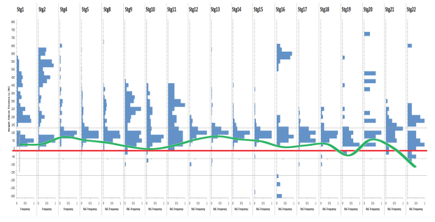
FIGURE 8

Microseismic Event Depth Histograms (29-Stage Bakken Well)

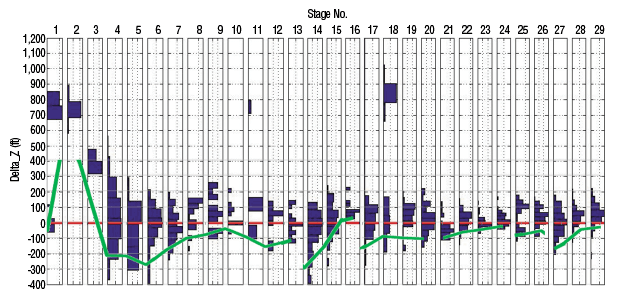
The results from the 29-stage well C (Figure 8) include obvious faulting effects. Stage 2 in the hybrid completion design included an 8- to 10-foot fault identified by geosteering. In this stage, points climbed to 900 feet above the zone of interest. As successive stages were pumped, the points came back to the borehole, indicating that fluid was being emplaced at the level of microseismic activity, and that the associated stress shadow in that interval was providing enough additional stress contrast to limit height growth in following stages.

This suggests that the process of multistage fracturing in a lateral is potentially a “self-correcting” process. When closely spaced fractures interact, they escape the stress shadow by propagating out of zone. Once enough stress has accumulated in the out-of-zone section, stress shadowing allows subsequent fractures to again be created in-zone. This probably explains why the emphasis on tighter stage spacing is proceeding in many unconventional plays without obvious problems.

However, understanding the impact of stress shadowing underscores the importance of using available means to keep fractures in zone and to minimize the additional hidden costs that can occur as more stages jump out of zone (deriving from, for example, the production of water from units outside the zone of interest).

Except for stages 11 and 18, which show some height growth related to faults or natural fractures, the rest of the stages in well C show a cyclical series of rising and falling steps. The 10,000-foot lateral was geosteered to remain within the Middle Bakken (the red line represents the top of the Middle Bakken layer). The histograms extend into the deeper Three Forks, and contact with this oil-productive zone may account for some variation in stage-to-stage production.

We expect that different stress profiles and different mechanical properties of the layers surrounding the borehole would lead naturally to differences in how the stages interact. While patterns from the Utica and Bakken plays are different, the basic observation of cyclical bounces in the microseismic activity seems to be common.

Rather than drilling many wells to separate the effect of a given completion strategy from the normal geologic variations that influence production, we believe microseismic analysis will make it possible to confidently determine optimal stage spacing for a given play with a reasonable cost/production improvement ratio.

Editor’s Note: The authors acknowledge Hess Corporation’s Bakken and Utica teams for their assistance in the hydraulic fracturing and microseismic monitoring analyses project referenced in this article. For more detailed information on the conceptual stress shadow analytical modeling solution or its application, see SPE 170924, a technical paper presented at the Society of Petroleum Engineers’ 2014 Annual Technical Conference & Exhibition, held Oct. 27-29 in Amsterdam.