Fracture Diagnostics

HOUSTON–While temperature logs have been a part of standard production logging packages for years, downhole fiber optic distributed temperature sensing (DTS) technology has introduced a more continuous measurement of both temporal and spatial temperature for diagnosing multistage fracture treatments in horizontal wells.

With fiber optic DTS measurements, downhole temperature can be measured during fracturing, shut-in and production to provide continuous and integrated information over the life of the well. Integrated DTS interpretation provides information on fracture/flow distribution to provide key insights into what happened during fracture treatments, identify problems in treatment design and execution, and improve the efficiency of multistage fracture stimulation.

The key component of using temperature measurements for fracturing diagnosis is the interpretation model. A new temperature interpretation model has been developed for fractured well diagnosis to understand flow distribution for multistage fractured horizontal wells using both DTS and conventional production logging tools (PLTs). It uses mathematical models built on mass, momentum and energy conservation of each component (reservoir, fracture, well completion and wellbore) in the system, and the components are linked through boundary conditions.

Using this approach, assumed properties of the flow field are input to generate pressure, velocity and temperature distributions. There are three steps in the interpretation procedure workflow. After initial evaluation to eliminate the nonproducing clusters and roughly assign the flow rate to reduce the computation time, the models are used to calculate the temperature distribution and compare the calculated temperature with the measured temperature. When the temperature is matched, the last step is confirming that the total rate interpreted is consistent with the surface-measured rate.

The core procedure in the interpretation workflow is the second part, local temperature matching. The objective is to match the simulation temperature with the measured temperature at each producing fracture location. This is performed independently fracture by fracture. A gradient-based inversion algorithm method is used to invert the flow profile from the temperature measurements.

Field cases from the Eagle Ford and the Marcellus shale formations illustrate how these models can be used to generate fracture/flow distribution in multistage fractured horizontal wells. The Eagle Ford well used temperature measurements from PLTs, and the Marcellus well used DTS measurements from a permanent fiber optic cable installed in the wellbore. The results show that temperature measurement is a comprehensive tool for fracture diagnosis.

Eagle Ford Case Study

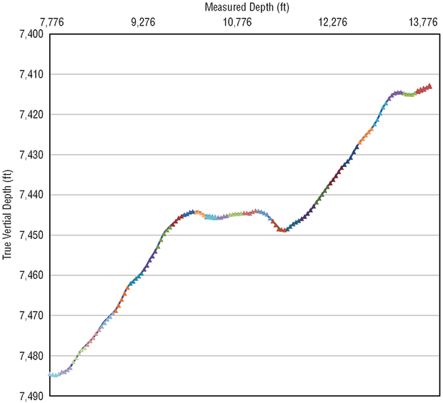
The interpretation modeling approach was first applied to interpret data acquired by PLTs during the production of an Eagle Ford gas well. The well was fractured with 15 stages and each stage had four clusters. The fracture spacing was 77 feet (75-foot cluster spacing with a two-foot perforating zone). Figure 1A shows the Eagle Ford well’s trajectory and Figure 1B shows the Marcellus well’s trajectory. Each triangle along the well represents the location of a perforation cluster and each fracture stage is color-coded.

FIGURE 1A

Eagle Ford Well Trajectory and Perforation Locations

 

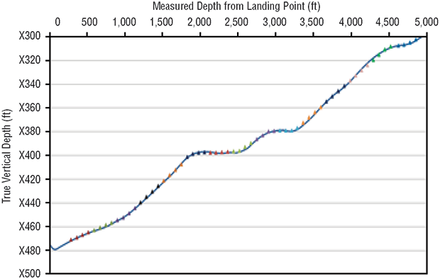
After the fracture treatment, the well was producing 1,600 Mcf a day. The water production rate was 160 barrels a day with a surface gas-to-oil ratio of 9,000:10,000 cubic foot/bbl. Since liquid production was less than 10 percent of the total volume according to the pressure-volume-temperature (PVT) properties, single-phase gas production was assumed for interpreting the temperature data. To account for the influence of liquid on heat transfer, the average heat conductivity based on the gas to oil ratio and water cut was used in the modeling.

The well trajectory made interpretation difficult. The flow in the wellbore is two-phase even though the reservoir is treated as a single-phase problem. The general upward trajectory with several low spots along the well results in complicated multiphase flow phenomena. The trajectory also directly influences the geothermal temperature at the wellbore location, which also is an important interpretation parameter.

During interpretation, only the fracture half-lengths were changed to match the measured temperature while all other parameters were kept constant. The parameters used in interpretation included 583 nanodarcy permeability, 4.2 percent porosity, 4,630 psi pore pressure, 0.56 gas specific gravity, 25 md-foot fracture conductivity, 25 percent fracture porosity, and 2,860 psi wellbore pressure.

FIGURE 1B

Marcellus Well Trajectory and Perforation Locations

The measured PLT temperature data are available from stages six to 15. During logging, two trips were made, and four sets of temperature data were available; two down passes and two up passes. The best dataset is the first down pass, where the wellbore temperature had not been disturbed by flow. If the first down-pass data have uncertainty, then the next pass should be used. In this example, the average temperature of all four passes was used.

Figure 2A shows the measured temperature data, as well as the geothermal temperature and simulation results. The geothermal temperature is calculated accurately based on the wellbore trajectory, and the calculated temperature is from a semi-analytical/trilinear modeling approach for a single-phase reservoir.

Temperature Changes

At the location of gas entry points at the perforations, gas enters the wellbore and expands, and the temperature decreases as a result of the Joule-Thomson effect. These temperature drops are observed in both the measured temperature data and the simulation results. The temperature drop in the curve is a combined result of the mixing of cool incoming fluid and upstream warm fluid.

FIGURE 2A

Simulation versus Measured Temperature Data

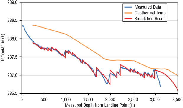
The simulation assumed instant temperature equilibrium, so the temperature drop is sharp. For the measured data, there is a mixing process that takes some distance for the temperature to stabilize. Also, the movement of the production logging tools causes some thermal dispersion. Therefore, the temperature drops in the measured data are smoother than the simulation result.

As the wellbore fluid flows from the toe toward the heel, fluid inside the wellbore is heated and temperature increases. Toward the heel, the flow in the wellbore is larger. During inversion, the parameter changed to match the measured temperature is the fracture half-length. Overall, the simulation result after inversion matches the measured temperature data well.

The magnitude of temperature drop at each perforation location indicates the amount of gas entering the wellbore, although the relationship is highly nonlinear. The well has no perforations from 2,291 to 2,370 feet. The temperature through this section increased, which correlates with the fact that no fractures had been created.

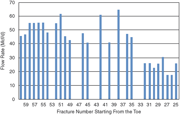
By matching the simulation temperature with the measured temperature, the flow rate distribution along the wellbore can be estimated. Figure 2B shows the flow rate profile results for each fracture from the temperature interpretation. The fractures are numbered from toe to heel. PLT data cover stages seven to 15, which correspond to fracture 25 to 60, so the interpreted flow rate profile is from fracture 25 to 60. The fractures with no flow rate indicate failed fractures.

This field case shows that temperature measured from PLT can be used to interpret flow distribution. For high-rate gas production wells, temperature data measured by PLT have enough resolution for interpretation. However, PLT temperature measurements are not continuous, and when running the logs, production has to be disturbed.

FIGURE 2B

Flow Rate Profile along Wellbore (Stages 7-15)

Marcellus Case Study

The second example illustrates using DTS data to interpret flow rate distribution from a Marcellus Shale well. The data were measured by a fiber optic sensor installed permanently outside the casing in the MIP 3H well, which is part of the Marcellus Shale Energy & Environment Laboratory (MSEEL) project near Morgantown, W.V.

The well was producing 1.83 MMcf/d of gas and 0.78 bbl/d of water at 180 days of production. Since the water production was minuscule, single-phase gas production was assumed for temperature data interpretation. The fracturing treatment had 28 stages, with four or five clusters per stage, for a total of 133 clusters.

FIGURE 3

Inversion versus Measured Temperature
And Inversion Flow Rate Distribution

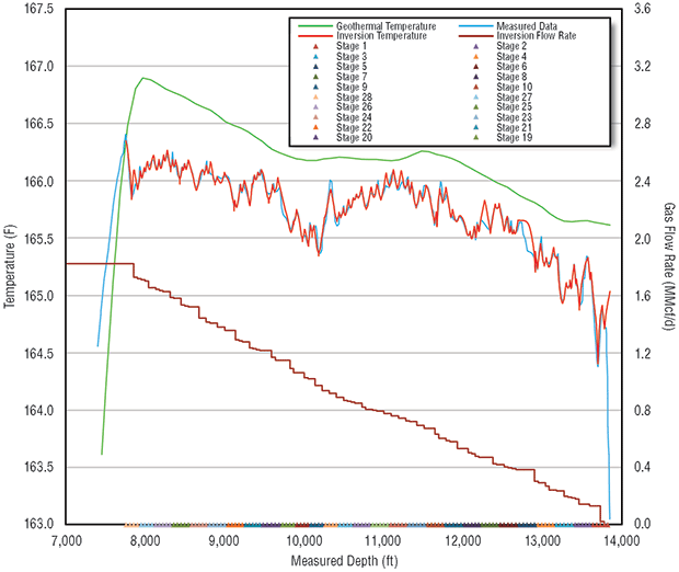
To improve interpretation efficiency, a strategy was applied to eliminate clusters that were not contributing to gas flow by examining the temperature derivative before interpretation. This can reduce the size of the problem that will be solved and save interpretation time. The measured temperature data are represented by the blue curve in Figure 3, which shows the inversion results from the second step in the modeling process. The inversion temperature, represented by the red curve, matched the measured temperature satisfactorily. The brown curve is the inverted production rate along the wellbore. The inverted total flow rate is 1.82 MMcf/d, which matches the measured total flow rate of 1.83 MMcf/d with a difference of 0.5 percent.

As noted, temperature decreases at the gas entry locations, but if a perforation location has no gas inflow, the temperature increases because the surrounding reservoir’s higher temperature warms the flow stream as it passes. This results in a negative temperature gradient from upstream to downstream.

Based on this principle, temperature derivative analysis indicated a positive gradient for 78 of the 133 clusters (60 percent cluster efficiency). The interpretation only needed to invert these 78 producing fractures, instead of all 133.

From the initial elimination, non-uniform initial guesses of flow rate were assigned to each producing fracture based on the magnitude of the temperature change. Figure 4 also shows inversion results from the second step in the modeling process. In this case, the initial flow rate guess for each fracture is shown along with the inverted flow rate profile for each fracture. It is observed that the middle stages (11-15) produce less fluid. The initial guess provides a reasonable estimation.

FIGURE 4

Initial ‘Guess’ and Inversion Flow Rate Profile for Each Fracture

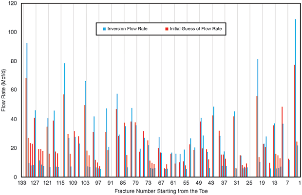
Since this set of temperature data is measured outside the wellbore, it was assumed that the temperature drop is not influenced by fluid mixing inside the borehole. Therefore, the production rate was assumed to be proportional to the temperature drop. Accordingly, a non-uniform initial guess of flow rate was assigned to each producing fracture based on its temperature drop compared to the geothermal temperature.

Well trajectory, completion and treatment execution all have strong impact on temperature behavior, and should not be overlooked when interpreting flow distribution. The benefits of using DTS measurements for flow interpretation is the temporal-continuous measurements, which can be used to confirm the interpretation, and importantly, confirm that the production from the well is not disturbed while measurements are made.