Process Control

BURLINGTON, MA.–Dynamic simulation of processes using rigorous models offers a wide range of applications for process engineering, process control, instrumentation, operation, training, and health, safety and environmental projects.

A key advance in dynamic simulation technology is developing virtual sensors that generate a process variable value–temperature, flow volume, pressure, composition, fluid properties, etc.–in real time by means of a rigorous dynamic model whereby the instruments are used to read the other available variables. Virtual sensors provide far more process variables than those that can be obtained from instruments, allowing any process to be monitored in much greater detail for better control.

Dynamic simulation of process plants and equipment is a very different discipline from steady-state simulation, in which time does not exist and the process plants are represented in a stable operational state–a state of equilibrium in which there is no accumulation of mass or energy. Dynamic models take time into account, along with the mass and energy imbalances that tend to occur in equipment. They are a type of simulation that set out to reproduce the real condition of a process plant, providing values that correspond to process variables as a function in time. They enable designers to interact with a dynamic model as they would with a real plant.

Dynamic simulation and steady-state simulation have developed along parallel lines, with solutions becoming ever-more modular, precise, interactive, fast, and easy to use. The main benefit of dynamic simulation is the much deeper knowledge it provides of the process as a result of improvements in system control design, plant operations, and staff training. Among the applications of dynamic simulation, some of which are used more extensively than others:

• It verifies the size and process layout. The size of the equipment used is determined by certain design rules covering the plant’s nominal operation. In some units, dynamic behavior depends on equipment size and process line arrangement. In such cases, it is necessary to carry out detailed dynamic simulations that verify the size and arrangement. One example is a compression train based on centrifugal compressors. The simulation has to verify that the design/size in question is capable of withstanding habitual movements (starting, stopping, operational change, etc.) without falling below the anti-surge line.
• It calculates flare load. Venting and flare networks undergo changes and additions during their lifetimes. This means constantly reassessing their real capacity and determining the real flows in the event of the safety valves blowing. API 521 recommends dynamic simulation for a more realistic assessment of the peak discharge flows, which often are lower than assumed. This typically obviates the need to readjust the size of the venting and/or flare collector, leading to major cost savings.
• It performs emergency system verification, and hazard and operability (HAZOP) studies. Emergency shutdown systems have a triggering logic defined by cause-and-effect matrices, or by a set of logical gates. A dynamic process model integrating this logic makes it possible to verify the design in the event of any triggering episode, and to determine the safest shutdown sequences. The dynamic model provides answers to many of the questions regarding HAZOP studies.
• It can perform basic control design/modification. The design of plants and equipment facilities is getting better from the steady-state point of view, with more integrated equipment and less inventory. This has been achieved at the expense of greater control complexity. This matter requires more in-depth study to ensure that the process can be controlled. Basic control structures are revised many times during a plant or facility’s lifetime, especially the startup mechanisms. Dynamic simulation has proven to be a useful tool in analyzing and modifying basic control structures.
• It is used in advanced process control. Developing model predictive control (MPC) controllers requires a more in-depth knowledge of the dynamics of the process, its interactions, causes of disturbances, linearity range, etc. At the heart of an MPC controller, there is a dynamic model based on response curves for each independent/dependent variable pair. If this model does not accurately reflect the process dynamics, the controller will not work properly. Having a rigorous dynamic model can help at certain stages of implementing an MPC controller project, especially in obtaining response curves that are difficult to achieve in a real plant. This will be conditioned by the cost/effort investment required to develop a rigorous dynamic model.
• It provides training systems for operators. Operator training systems (OTS) are perhaps the best known and most widely used dynamic simulation application. Similar to flight simulators for pilot training, OTSs often are required for training operators and technicians, especially for those responsible for remote assets such as oil and gas platforms. OTSs also are required for plants that have been in operation for many years and are in need of improving training procedures for emergency situations, or for infrequent critical scenarios.

In addition to these applications, there is another area of dynamic simulation that is less often used, but that can offer added value: creating virtual sensors, also known as soft sensors or online inferential models.

Virtual Sensors

A virtual sensor is capable of estimating an important and often difficult to measure process variable such as a product quality. It does this by means of an online calculation using other measured variables. There are two fundamentally different types of virtual sensor:

• Steady-state, which are constructed on the basis of calculations in which the time variable plays no part, since the process is either of a nondynamic nature or the dynamic effects are negligible; and
• Dynamic, which are based on calculations in which time and the effects of integration are taken into account.

Virtually the entire process industry uses more or less complex virtual sensors to calculate the mass and/or energy balance in the control systems themselves. A typical example is the mass and energy balance in an exchanger, with a view to calculating an unmeasured exit temperature. This calculation can be as complicated as is necessary to take account of the effects of pressure and temperature on calorific capacity and density, all the more so if the fluid’s analytical composition is known. These calculations often are so complex that they can be deciphered only by the calculation’s author, which means they become meaningless when the author moves to another job.

Using steady-state or dynamic simulation models can help when it comes to developing calculations and correlations that thereafter are executed online, or simulation models that can be used directly online on the basis of real-time process data.

The term online can be interpreted in a number of ways. In this case, it refers to automatically obtaining data from a plant in real time, performing a calculation by means of a correlation or model, and subsequently exporting the value to the plant’s control or information system to inform the operator or serve as a controller’s input signal.

However, we should not expect a dynamic simulation to be capable of providing acceptable virtual sensors for any process unit. Its application range is limited to units that meet the following criteria:

• Circulating components are known or well measured.
• The thermodynamic packages for these components are reliable.
• The plant’s unit operations are well represented by a simulator. One example is a distillation column whose reaction units require a degree of knowledge that is seldom available.
• The processes’ main disturbances are measured.

FIGURE 1

Parallel Heat Exchangers Diagram

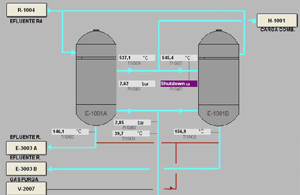
Parallel Heat Exchangers

Consider the case of a steady-state virtual sensor that calculates, among other things, the fouling of two parallel shell and tube exchangers (Figure 1). What circulates on the tube side is a reactor exit gas stream; on the shell side, a stream of entry gas circulates in these same reactors. Their purpose is to preheat the combined reactor load from 40 degrees Centigrade to 540 degrees, taking advantage of the reaction exit effluent, which is at 650 degrees. These exchangers tend to become fouled over time. To be able to program and justify the cleaning operations that involve a plant shutdown, it is important to know with some precision the degree of fouling and its extent.

The plant has online composition analyzers for both streams, which in conjunction with data from other instruments (pressure, temperatures, total flow rates), are collected automatically by a rigorous steady-state model that filters the data, closes mass and energy balances, and on that basis calculates the degree of fouling. The system also obtains supplementary data such as convection factors, densities, etc.

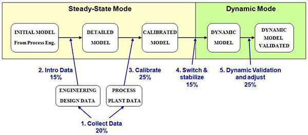
Figure 2 shows the construction stages of a dynamic model and its corresponding effort in percentage terms, with respect to the total time required for development.

FIGURE 2

Dynamic Modeling Workflow

Once the dynamic model has been constructed, the most important stage is its dynamic validation. This consists of verifying that the model dynamic is the same as that of a real plant, given the same inputs and under the same boundary conditions. Often, not enough attention is paid to the latter part of the process, since the model is assumed to be good because it is based on a rigorous simulation tool, or because the steady state is represented correctly.

Traditionally, rigorous dynamic models have been viewed with a certain amount of scepticism when it comes to reproducing real-plant dynamics. This scepticism is, nevertheless, understandable, as hardly any studies have been published that demonstrate accuracy.

There are three ways to carry out a complete dynamic validation. The first is comparing movements. This relates to effecting a change in the real plant while the other actions remain constant, and then repeating the same change in the model to determine whether it produces the same dynamic and effects. This means of validating a model could not be carried out easily in reality because the disturbances (whether measured or unmeasured) are acting on the process also. It is difficult to obtain clear responses in most cases, although for some very simple models, the responses may be sufficient.

The second way to accomplish dynamic validation is to compare dynamic matrix control (DMC) models. In this case, step-tests are conducted on the simulation model to identify a DMC model that can be compared with a real plant. Logically, this is possible only if a reliable DMC model of the unit exists in the first place.

It is important to stress that this type of comparison does not take into account the offsets of the simulation model in comparison with the real plant, so it only compares process gains and dynamics. These may be sufficient if the aim is to obtain response curves.

FIGURE 3

Empirical DMC Model Fitted to Real Plant Data (Blue) versus 
Rigorous Dynamic Simulation DMC Model (Red)

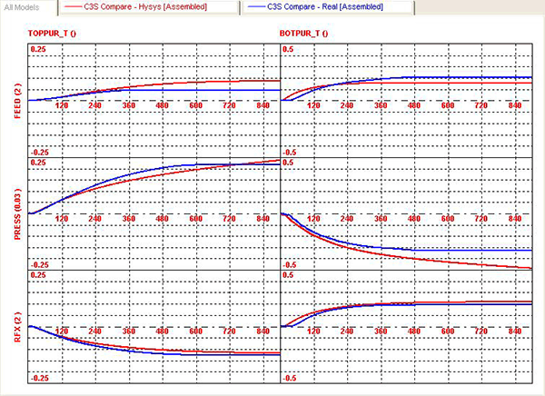
Figure 3 shows an example of comparing DMC models for a propane/propylene splitter containing 230 sieve trays and a heat pump. It compares feed, pressure and reflux response curves with top and bottom quality. Marked in blue are the curves obtained from step-tests on the real plant; the red shows responses obtained from the simulation model’s step-tests.

The third option is comparison with historical data. This involves running the dynamic simulation against a set of historical data from the real plant. Once the validation period has been chosen, all the events that occurred in the real plant–operator actions, MPC actions, measured disturbances–are introduced synchronically into the dynamic model in order to compare the variables calculated by the dynamic model with those obtained from the real plant.

This type of validation is useful only if the main disturbances in the real plant are measured. Strong disturbances that go unmeasured cannot be introduced into the simulation model; consequently, the responses may be different.

Propane/Propylene Splitter

Comparing historical data was used to validate a case study example from a propane/propylene splitter unit. It consisted of two heat-integrated columns, where the condenser of the first was the reboiler for the second. This introduced a heat integration interaction that complicated the dynamic responses.

FIGURE 4 

Cooling Water Temperature (FF3) and Feed Temperature (Scale = 10-30 Degrees Centigrade)

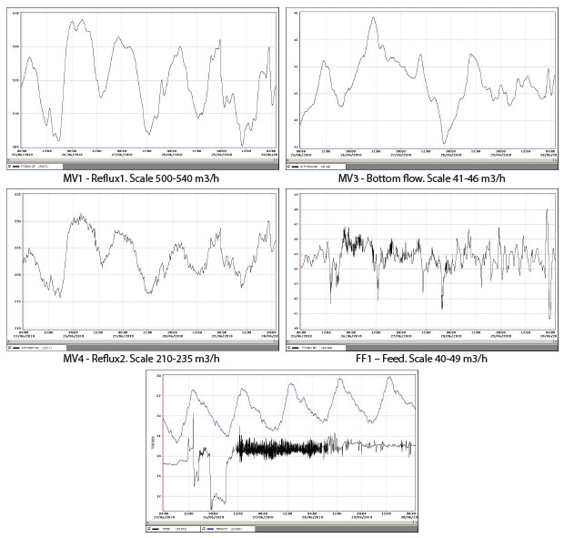
FIGURE 5A

Percent of Propylene in Propane at the Bottom of the First Column

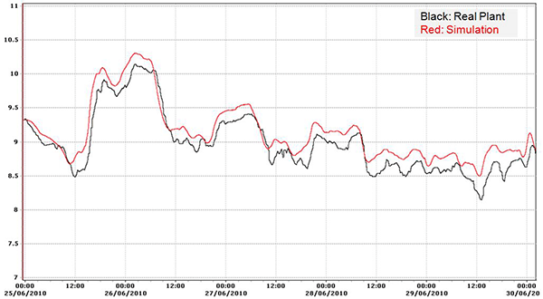
FIGURE 5B 

Percent of Propane in Propylene at the Top of Second Column

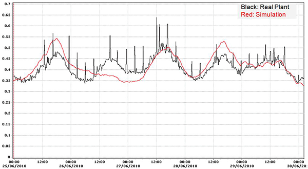
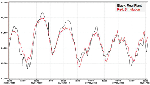
FIGURE 5C

Differential Pressure of Second Column

The validation period for the historical data variables with which the dynamic model was supplied was five days at one-minute sampling, and the propane-to-propylene ratio was measured upstream by an online analyzer, meaning the ratio was used as one of the boundary conditions. The charts in Figure 4 show the trend of actual plant variables imposed on the simulation model.

Figures 5A-5C show some of the variables calculated by the dynamic simulation model (shown in red), compared with the corresponding variables of the real plant (shown in black). Specifically, Figure 5A shows the percentage of propylene in propane at the bottom of the first column; Figure 5B shows the percentage of propane in propylene at the top of the second column. It is important to bear in mind that the scale is 0.0 to 0.7 percent, and it is a polymer grade quality, where impurity must not exceed 0.5 percent. Figure 5C shows the differential pressure of the second column. The pressure is floating in both columns, and there is no associated control loop.

Matching the differential pressure values could be the basis for developing a virtual sensor capable of providing a simulated differential pressure value that would not take into account the phenomenon of flooding, since the simulation tool used doesn’t represent the flooding effects. Therefore, it could be used to prevent flooding when the variables–real versus simulated–indicated a large difference.

Rigorous simulation models can offer a way forward for developing virtual sensors. Those based on steady-state models have a wide range of applications, and could be used to develop a correlation or they could be used online.

Dynamic models, for their part, can provide reliable values for dependent time variables, but their range of uses is restricted to certain specific cases. Their main weakness is the lack of precise knowledge concerning the composition of the entering stream(s), for which online analyzers might be required.