LITTLETON, CO.–Those of us who grew up with Lionel trains imagined our powerful, steaming black engines transporting people, lumber, coal and other cargo–but probably not sand. A point of fact is that Lionel did indeed make a scale-model hopper car for imaginary shipments of sand, iron ore and other such cargoes, but what kid dreamed of running the rails with carload after carload of sand in tow?

The boom in hydraulic fracturing has created a new rail industry for the transportation of frac sand or equivalent ceramic proppants to plays such as the Marcellus, Bakken and Eagle Ford, and for good reason. Multistage fracturing operations in shale gas and tight oil plays require enormous volumes of proppant–millions of pounds in each horizontal well. From mines in Wisconsin, Illinois and Minnesota or shipping terminals in Texas, Washington and California, real and artificial sands are being shipped by boxcar to well sites all across the United States.

Sand, either mined or manufactured, is the lifeblood of unconventional (and increasingly) conventional plays in basins such as the Permian. With slick water or gel mixtures opening the fractures, large quantities of various mesh sizes of sand or ceramic proppants are required to prop open the fractures to maintain oil and gas flow through the created wedges and back to the well bore.

The total volumes of frac sand pumped per well vary according to the play, and the lateral length and the number of frac stages per lateral. In the Bakken/Three Forks play, wells are reported to typically average between 2 million and 4 million pounds, while Marcellus horizontals can require 5 million pounds or more of proppant.

The Eagle Ford Shale is arguably the most geologically complex unconventional play in North America, and field development complexity is manifested in a high degree of well-to-well production variability across the play. A typical Eagle Ford horizontal well has a 5,000-foot lateral length and is hydraulically fractured in 15 stages using between 50,000 and 150,000 barrels of water/gel and between 1 million and 11 million pounds of sand.

FIGURE 1

Eagle Ford Well Lateral Lengths, Number of Frac Stages, and Proppant and Fluid Volumes (Colors Represent Different Operators)

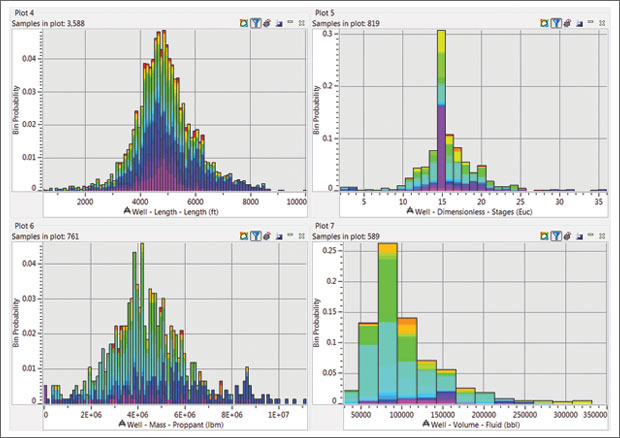
Figure 1 shows the range of well lengths, number of fracture stages, proppant and fluid used for wells in the Eagle Ford play. The histogram counts are colored to illustrate different Eagle Ford operators, highlighting a wide diversity of engineering approaches.

By The Numbers

With a typical rail car able to carry 200,000 pounds of sand, and an average Eagle Ford well using 4 million pounds of proppant, 20 rail cars full of sand are required for one Eagle Ford fracturing operation, with more heavily treated wells requiring more than 50 rail cars. Extrapolating across the lower-48, nearly 110,000 rail cars of proppant were delivered to well sites in the last quarter of 2012 to support fracturing operations.

Assuming a delivered sand price of $0.10 a pound, roughly one-third of this cost is driven by rail charges and one-fourth by transloading and trucking, leaving the remaining 40 percent associated with direct sand costs. This translates to a price range difference of $400,000 to $1 million between an average and high-proppant well in the Eagle Ford. With more than 3,500 wells drilled since 2008, the nearly 10-fold variation in proppant levels indicates the complexity of trading proppant volumes and current costs for longer-term well performance.

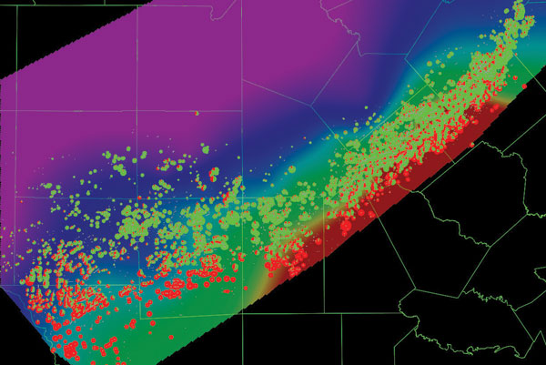
FIGURE 2

Map of Initial Well Production with Major Rail Lines in Orange (Red = Natural gas; Green = Condensate and Oil)

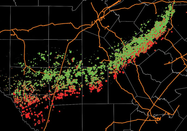
A recent study has accessed a wealth of public oil and gas data for the Eagle Ford play from the Texas Railroad Commission. Mapping initial well production rates across the play illustrates the range of performance and the transition from natural gas to oil production across the Eagle Ford trend, as shown in Figure 2. In this map of initial well production, red denotes natural gas and green denotes condensates and oil.

Covering an area of more than 11,000 square miles, Eagle Ford production exceeds 1 million barrels of oil equivalent a day (with approximately 70 percent liquids) from more than 3,500 fractured horizontal wells. The Eagle Ford is grossly a depth-driven petroleum resource. It produces oil at depths of 5,000-8,000 feet to the northwest, grading through condensate and natural gas liquids, to dry gas at depths of 10,000-12,000 feet to the southeast. Initial production rates range from more than 6,000 barrels of oil a day to more than 20 million cubic feet of dry gas across the dip trend. Maximum oil production, in general, is found to correspond to regions with lighter API gravities of 40 degrees up to the condensate transition of 45 degrees.

FIGURE 3

Production Variability for Regional Sampling of Eagle Ford Wells (Colors Represent Different Operators; Inset of Well Production Range by Operator)

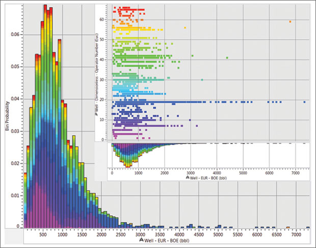
Converting natural gas production to barrels of oil equivalent provides a basinwide perspective of relative well performance. Figure 3 shows the production variability for a regional sampling of Eagle Ford wells, colored by operating company, with initial oil, gas and liquids production converted to boe. Mean daily initial well production is 886 boe, and maximum production is approximately 7,300 boe. The inset image of Figure 3 illustrates the variability in well production for all Eagle Ford operators, leading to the question of whether well engineering or location is more important.

Optimizing Proppant Volumes

In 2013, industry capital expenditures in the Eagle Ford are expected to approach $30 billion. There are about 240 rigs active in the play, down from a 2012 peak of more than 260 rigs. With efficiencies gained from pad drilling and greater drilling productivity, this level of activity can add 250 new wells every month, ready to pass off to completions engineers for hydraulic fracturing. Translating back to sand usage, this places a demand for roughly 500,000 tons of proppant a month, the equivalent of 5,000 rail cars!

That is obviously a lot of train activity driven by only one aspect of Eagle Ford development: fracturing. But is all that sand really necessary? How can operators determine an optimal amount of proppant, and how much sand is too much?

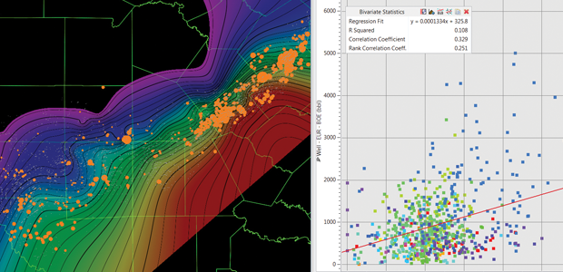
FIGURE 4

Production Response to Proppant Volume (Left = Production Divided by Total Proppant on Well Depth Background; Right = Cross-Plot of Production versus Proppant)

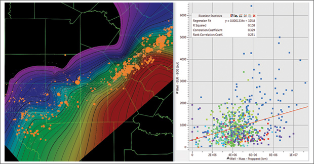
Details of specific proppant sizes or types are sparse in the public domain. However, available information shows a wide range of mesh sizes are deployed by different operators. What is the impact of these millions of pounds of proppant on well production levels? Figure 4 provides two perspectives of production response to proppant volume. At left is a map of well production divided by total proppant (yellow bubbles) on a background of well depth. At right is a cross-plot of well production (boe) on the vertical axis versus proppant (millions of pounds) on the x axis, colored by Eagle Ford operator.

These statistical perspectives illustrate the variable impact of completion size on production, with a moderate level of correlation (»0.366), but a large regional variation. In particular, the big producing wells to the northeast (in Karnes and Gonzales counties) respond best to proppant levels. This amplifies the question of whether well performance is driven more by engineering drilling and completions or location (i.e., geology).

Unraveling Complexities

Simple statistics result in ambiguous results. A multivariate analytic approach is required to unravel the complexity of the effects of drilling and completions engineering–and geologic conditions–on well production. Linear multivariate statistics are too simplistic to model the diminishing returns (i.e., nonlinear relationships) of reservoir thickness and size of completions, with bigger not always being better. Neural networks can provide a nonlinear option for modeling these reservoirs, but they do not provide sufficient insight into the effect of different parameters and properties to drive an optimization strategy.

A nonlinear, multivariate analytic technique based on transforming variables into linear predictors of production has proven to be a robust and reliable approach for assimilating and understanding the constraints for unconventional well production. Comparing analytic models using engineering only, and engineering and geology, illustrates the trade-offs between how wells are drilled and where.

FIGURE 5

Predicted Production using Engineering Data Only (Left) versus Engineering/Geologic Data (Right)

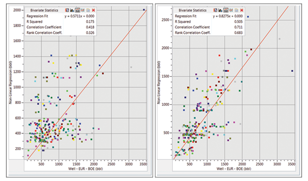
Figure 5 shows nonlinear production predictions based on engineering data only at left and engineering and geologic data (including depth and thickness) at right. More accurate predictions and less uncertainty are attained with a balanced engineering and geologic model.

In the Eagle Ford, analytics reveal that well depth is one of the largest drivers of well production–directly related to the lightness of the petroleum (i.e., more likely dry gas or condensate) and pressure. From an engineering perspective, horizontal well length, number of fracture stages, amount of fluid and, yes, proppant volumes are among the important determinants of well production.

FIGURE 6

Predictor Transformations Highlighting Range of Parameters and Properties Corresponding to Best Production

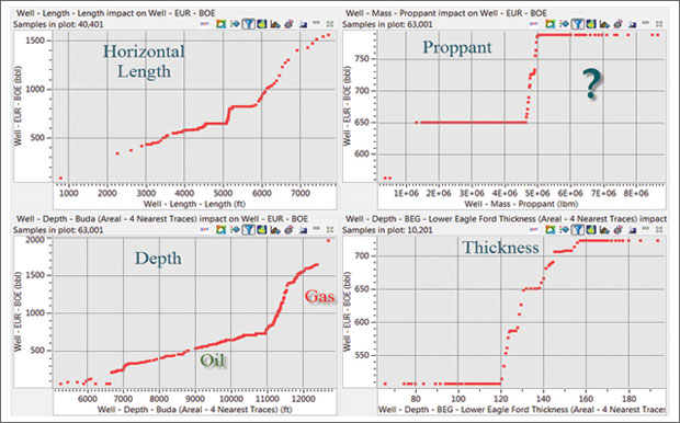
Figure 6 provides insight into how engineering and geology interplay to drive well production. Well length and well depth are undoubtedly the biggest and nearly linear drivers of well production. The thickness of the Eagle Ford matters, to a point, beyond which hydraulic fracture effectiveness does not fully exploit reservoir thickness. Interestingly, the number of fracture stages and total fluid pumped have the strongest correlation with production, while proppant, as visualized, has a less certain impact on production.

These analytic results echo the ongoing debate in the Eagle Ford with respect to the optimal deployment of proppant. While bigger generally appears better, there is a lot of complexity related to petroleum phase (oil/gas/condensate), fluid/proppant ratio, type of fluid, and the blend of different mesh sands during the course of hydraulic fracturing.

Taking a global perspective across the entire Eagle Ford, there is no clear statistical indication that treatment levels above 5 million pounds are more effective. Although massive proppant deployments appear effective in the light oil regions of Karnes and Gonzales counties, more moderate and customized proppant usage appears effective in the natural gas and western regions of the Eagle Ford.

Comprehensive Model

The combination of engineering and regional geologic information provides some interesting perspectives on Eagle Ford sweet spots and optimized well parameters. However, a challenge for field development in this play is locating faulting and fracturing trends, and other geologic features conducive or hazardous to hydraulic fracturing. Seismic data are particularly useful for mapping a number of detailed geologic constraints in the Eagle Ford play, including depth, thickness, fault locations, fracture trends and orientation, and rock fracturing characteristics.

FIGURE 7

Fault Proximity Seismic Volume

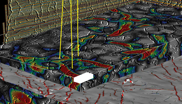
Figure 7 illustrates the application of a threshold set to a fault probability volume, which is then used to estimate well bore proximity to the nearest fault. Color intensity indicates the distance to the nearest likely fault. The nearest or average distance to a likely fault is then extracted to each well bore intersecting the seismic volume. For this study, seismic data provided by Global Geophysical provided detailed insights into geologic influences in McMullen and LaSalle counties.

Fault proximity, and other seismic attribute volumes or maps, can be extracted along every well bore path in the survey area. Using the same nonlinear techniques, detailed well production performance analysis can be performed, making use of well-based engineering and geologic data, and extracted seismic information. The result is a better predictor of well performance, with engineering, regional geology and local geology all considered.

Estimates can be made of the minimum distance a well bore can be safely drilled and completed near a fault. This information is essential for optimized planning; after hauling tons of sand 1,000 miles by rail, the last thing operators want is to have hydraulic fluid and proppant escape along faults!

Finding The Balance

The combination of engineering, geological and geophysical data produces a comprehensive and highly correlated model of well production. Regional models can be created using drilling and completions engineering data and well-log driven estimates of depth, thickness and rock properties. Complementary localized models can be created using regional data enhanced with detailed seismic measurements of rock strength and brittleness, fault proximity, fracture trends, and more.

Predictor transform plots are analyzed to provide insight into how specific parameters and properties affect relative well production (Figure 6). Specific observations for data across the Eagle Ford are that wells with 5,500-foot laterals and fracture spacing of roughly 300 feet (i.e., 18 fracture stages) that deploy approximately 100,000 barrels of fluid and 5 million pounds of proppant are likely better producers. These observations vary with the type of production metric (e.g., boe of oil/gas/condensate versus oil) and length of production window (e.g., initial production versus 90-day production).

From a geologic perspective, deeper Eagle Ford targets generated more boe because of lighter petroleum and higher pressure, while a reservoir thickness of about 150 feet appears to be a good threshold for sweet spot identification.

With a reliable and explainable nonlinear prediction model in place, a normalization of the engineering parameters can be performed by selecting nominal average values for well bore length, fracture stage length, etc., across the entire Eagle Ford.

FIGURE 8

Relative Production Sweet Spot Map

The result of this workflow step was a production sweet spot map, indicating expected relative well production if all well engineering was held constant (Figure 8). In other words, a map was created to indicate what the rocks likely would produce if every well was drilled and completed the same way.

There will continue to be a lot of freight trains moving a lot of sand across the rails in South Texas, no matter how one looks at Eagle Ford geology and completion design. However, the ability to use analytical techniques to understand key productivity variables and better predict well performance can allow operators to focus their investments in those areas with the highest potential, and ultimately, focus their development strategies and well designs to optimize the balance between initial well cost and long-term performance metrics.