Enhanced Oil Recovery

GOLDEN, CO.–While initial production rates are high from horizontal wells in ultratight oil formations, reservoir recovery factors are very low, averaging in the range of 5-10 percent. The low primary recovery factors are largely the result of the ultralow matrix permeabilities. And, unlike conventional reservoirs, in which waterflooding is the main choice for improving oil recovery by providing pressure support and sweeping oil to production wells, waterflooding does not appear to be a viable secondary recovery option in shale oil reservoirs because of low permeability/injectivity.

Beyond primary artifical lift, gas injection may be an effective alternative for improving recovery rates in tight oil reservoirs such as the Bakken Shale, where the source rock and the reservoir rock are one and the same, and permeabilities are measured on the microDarcy scale. A Colorado School of Mines study examined a four-section area of the Elm Coulee Field in eastern Montana to evaluate the impact of three gas injection schemes: carbon dioxide, immiscible hydrocarbon, and miscible hydrocarbon.

A flow simulation model was used to examine the difference in total recovery, production rate and efficiency. Recovery efficiency was similar for both miscible hydrocarbon gases and carbon dioxide, with recoveries increasing from 6 percent on primary production to around 20 percent with gas injection. While the increased recovery was encouraging, both methods have some practical limitations. For instance, the availability of CO2 is limited in many unconventional basins, and while hydrocarbon gases are a byproduct of production in most tight oil fields, their marketable value can preclude using them as injectants for EOR (assuming gas infrastructure is available).

The study demonstrates that injecting gas (both immiscible and especially miscible) will increase oil recovery appreciably in very low-permeability reservoirs. Given the size of the resource base in the Bakken, Eagle Ford, Niobrara and other liquids-rich plays, a large prize is available to those who find ways to increase recovery from tight reservoirs.

In the case of injecting produced gas to enhance oil recovery, the economics certainly can be favorable, even with the recovery in natural gas prices, particularly in the case of associated produced gas with limited local processing or take-away capacity (as is often the case in the Bakken). To assess the economics, a cost/benefit analysis was performed to compare selling the gas with injecting it to increase oil production. Assuming a $10 million investment in compression and facilities for the four-section Bakken study area, the net present value was $68 million with a return rate of 83 percent at an average gas cost of $5 an Mcf and a conservative oil sales price of $80 a barrel.

At present, the United States is producing more than 300,000 barrels a day from gas injection projects. Gas injection tends to work well in higher-pressure (deeper) reservoirs and those with higher API gravity oils. Unconventional shale oil reservoirs tend to have both of these characteristics, in addition to ultralow permeabilities. While gas injection appears favorable for EOR in unconventional oil reservoirs, the ability to inject produced hydrocarbon gases as an effective alternative to CO2 will be key to long-term recovery efforts given carbon dioxide’s limited availability in plays such as the Bakken Shale.

Reservoir Modeling

FIGURE 1

Map of Elm Coulee Field
With Modeling Sector Highlighted

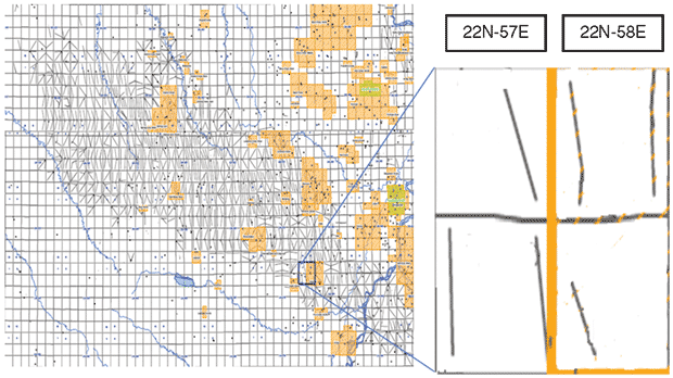
The Elm Coulee Field study evaluated the performance of the three solvents for gas flooding using a numerical reservoir simulator. A section of the field was selected for reservoir modeling in previous work using a commercial finite difference simulator to evaluate well placement and injection scenarios (Figure 1). The structure and dimensions of that model, along with rock and fluid properties, and the optimum well development and injection strategy, were used for this study.

The modeled sector is two miles long by two miles wide and located in parts of townships 22N-57E and 22N-58E. It consists of 10, single-lateral horizontal wells (six of which were historical wells and four of which were added in the previous study for the optimal gas injection scenario). The reservoir section was divided into 53 grid blocks in the x direction, 53 grid blocks in the y direction, and eight grid blocks in the z direction. The grid blocks were 200 feet in length in the x and y directions, and three feet thick in the z direction, resulting in a 24-foot pay zone.

At this location, it was assumed that the overlying shale layer contributes to oil production, and the pay zone consists of the upper shale and dolomite regions of the Bakken formation. The top three layers in the reservoir grid represent the upper shale zone, and the bottom five layers are the dolomite. The shale occurs at a subsea level depth of 7,500 feet.

Both the upper shale and middle dolomite members of the formation were modeled with a homogenous porosity of 7.5 percent. The shale layers contain natural fractures that formed during the kerogen conversion process, followed by oil generation and expulsion. Log analysis shows that these natural fractures provide 6-8 percent porosity in the shale. The dolomite porosity is in a similar range.

The results of pressure buildup tests indicated a permeability value of 2.5 mD in the upper shale region. However, the capacity to transmit fluids of the natural fractures present in these layers depends on pressure. As reservoir pressure drops with production, permeability decreases in the shale layer. The phenomenon of pressure-dependent permeability is incorporated into the model’s upper shale using permeability multipliers. The dolomite region is 15 feet thick with a permeability value of 0.015 mD. The permeability in this region is not affected significantly by pressure changes. A vertical-to-horizontal permeability ratio of 0.01 was used for both members of the reservoir.

Because of the very low permeability values, the hydraulic fractures created have very large permeability values. At the time the wells were drilled, there was still debate about the most effective types of fractures, namely longitudinal (along the wellbore) versus transverse (perpendicular to the wellbore). These wells were drilled in the direction of maximum stress to create longitudinal fractures.

In the model, the hydraulic fractures were placed along the path of the horizontal wells in the longitudinal direction, and were represented as zones of increased permeability in the grid that could extend tens of feet from the wellbore. Therefore, the permeability of grid blocks with a well was increased to 100 mD.

Another interpretation was to assume a representative grid block permeability for the hydraulic fracture permeability. In this case, fractures were represented as zones of increased permeability around the wellbore. Fractures were assumed to be approximately one-eighth inch wide with a permeability of 1 million mD. Therefore, a 200 foot-wide grid block would have an average permeability of 100 mD.

Production Modeling

FIGURE 2

Two-Dimensional View of Reservoir Grid
With 10 Well Locations

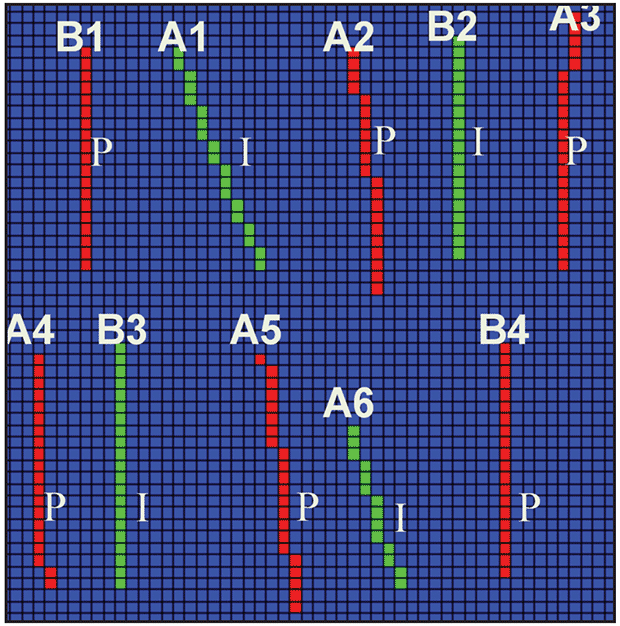
The reservoir oil in this region of Elm Coulee has an API gravity of 42 degrees and the gas gravity is 0.95. The estimated oil in place is 5 million barrels per square mile, with a sectorwide model covering a four square-mile area. The simulated output of the sector model provided an oil-in-place value of 19.96 million barrels.

Figure 2 shows the locations of wells in the model. The six original single-lateral horizontal production wells (A1-A6) had produced on primary production for 39 months. Four additional wells (B1-B4) were included in the model to optimize the gas injection strategy. Since the wells were originally drilled to penetrate the Middle Bakken, the completion interval is in the sixth layer of the reservoir grid (the middle of the dolomite).

FIGURE 3A

Well No. A5 Historical and Simulated Production Data

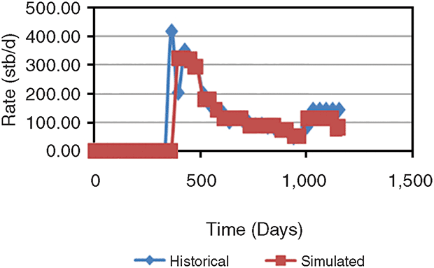
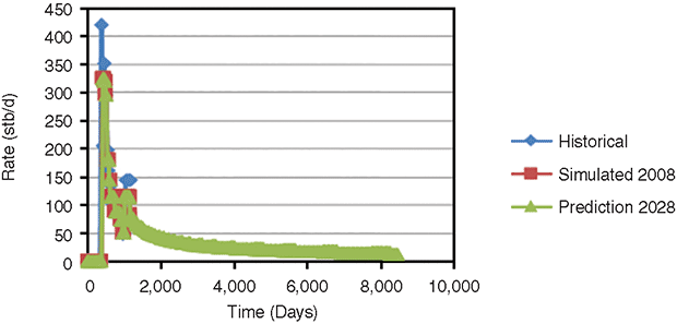
Figures 3A and 3B show the results for one of the six wells during primary production. When the original wells were on primary production, the oil rate was constrained to reproduce the historical production data (Figure 3A). A base case primary production prediction model was then run with the wells pressure-constrained to match the typical decline curve behavior (Figure 3B).

To evaluate the behavior of the reservoir on primary recovery and compare it with the gas injection cases, the model was run for 20 years after the 39 months of primary phase production. The total sector output for primary recovery was 1.2 million barrels. Note that the declining production trend emphasizes the need for implementing an EOR operation in this tight oil reservoir.

FIGURE 3B

Well No. A5 Predicted Production Data

The first model injected a hydrocarbon gas that was immiscible with the reservoir oil. This was achieved in the model by turning off the miscibility of the injected gas with oil so that gas formed a separate gas phase in the reservoir. The second model evaluated injecting a hydrocarbon gas that was miscible with the reservoir oil. The properties of the injection gas were set to equal the produced gas composition.

The third model represented CO2 injection. An extension of the black oil model, it consisted of four components: water, oil, reservoir gas and solvent. It was based on the assumption of first-contact miscibility between the hydrocarbon components and CO2. Displacement was dominated mainly by a miscible regime because reservoir pressure did not fall below bubble-point pressure and was maintained near or above thermodynamic minimum miscibility pressure (3,100 psi).

For all three models, gas was injected using the same four wells (A1, B2, B3 and A6, with the remaining six wells serving as producers) and the same bottom-hole pressure constraint target value (6,000 psi).

Injection Scenario Results

In the first scenario (injecting an immiscible produced gas composition that was not allowed to dissolve back into the oil phase), the gas saturations increased near the injection wells and pressure increased significantly (Figure 4). Daily injection rates ranged between 80 Mcf and 225 Mcf, and the total amount of gas injected was 3.78 x 106 Mcf, equal to 0.054 of the pore volume (PV).

FIGURE 4

Pressure Map of Middle Layer
After 20 Years of Immiscible Gas Injection

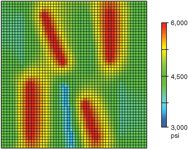
This injection scenario showed increased recovery from all six production wells a few months after starting injection. However, the increase was minor and held steady for the 20 years of injection. This is because immiscible injection only provided pressure support to the reservoir and did not initiate any oil displacement benefits (i.e., an oil bank was not formed and residual saturations were not reduced). Even so, the 6.02 percent calculated recovery factor during primary recovery was more than doubled to 13.3 percent with immiscible gas injection.

In the second scenario (injecting a hydrocarbon gas that was miscible with the reservoir oil), injection rates ranged between 150 Mcf/d and 600 Mcf/d, accumulating a total PV of 0.18. The production rates from all six horizontal producers increased one to two months after initiating injection. The highest field production rate occurred after five years of injection at 678 bbl/d, and the cumulative recovery at the end of 20 years was 4.26 million barrels.

FIGURE 5

Oil Saturation after Miscible Gas Injection

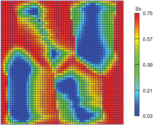
The recovery factor was calculated at 21.3 percent, or 15.3 percent higher than during primary production. Solvent breakthrough occurred after 3.6 years of injection. Figure 5 shows that the oil saturation is much lower in this scenario than with immiscible gas. The miscibility allows the displacement mechanism to reduce the residual oil saturation, which translates to higher production rates, better sweep and greater cumulative recovery.

CO2 injection results were similar to the miscible gas injection case, even though the properties and miscibility of the injection gases were different. CO2 injection rates ranged between 170 Mcf/d and 700 Mcf/d, which was equivalent to 0.20 PV.

FIGURE 6

Sector Production Rates
(Primary and Three Injection Scenarios)

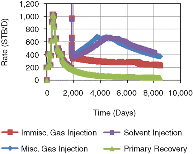
Increases from the production wells were observed after one month of injection, with the highest rate of 672 bbl/d occurring eight and a half years after starting injection, which was much later than with miscible gas injection (Figure 6). The recovery factor was only slightly higher (21.58 percent, or 15.6 percent higher during the primary phase). In this case, solvent breakthrough occurred 5.4 years after initiating injection.

TABLE 1

Three Injection Scenario Results

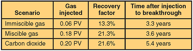
While the modeled results show similar recoveries for CO2 and miscible gas injection, 10 percent more CO2 was injected into the formation than miscible gas to recover only 0.003 percent more oil (Table 1). Moreover, the peak production rate was slightly delayed for CO2, and injection and gas breakthrough time occurred later. These differences likely were related to the ease of hydrocarbon gas miscibility compared with CO2 miscibility.

Economic Considerations

Simple economic cases were developed to evaluate the hydrocarbon injection scenarios. While produced gas can be sold to improve the tight oil project economics in many cases, this analysis compared the value of using the gas to increase oil recovery versus the value of selling the gas volumes. Obviously, produced hydrocarbon gas must be compressed before it is reinjected into the reservoir. The initial investment for the compressors was assumed to be $10 million. In addition, 10 percent of the total injection gas volume will be needed to fuel the compressors.

In the four-section Bakken study area, there would not be enough gas produced to supply all of the gas needs, so additional makeup gas must come from other sources or areas of the field. In this analysis, the cost of fuel and injected gas was $5/Mcf (either in the form of lost revenue or purchase cost) and the pre-tax value of each incremental barrel of oil was $80.

For the immiscible case, the economics appear favorable. The internal rate of return was 51 percent with a 2.4-year payout. Using a discount rate of 10 percent, the net present value was $30 million for the Elm Coulee study area. For miscible produced gas, the results are much better, with an NPV of $68 million, a 1.7-year payout, and an 83 percent rate of return. Although many simplifying assumptions were made in this economic forecast, it does illustrate that injecting hydrocarbon gases has significant potential in tight oil reservoirs from both a technical and economic standpoint.

Gas injection in the Bakken and other shale oil reservoirs looks promising, particularly for miscible gas. Gas injection is a viable option for increasing recovery factors above the 5-10 percent that is observed from primary production in these plays. Importantly, this study demonstrates that significant oil can be recovered, regardless of the type of gas injected. Even if the gas is not fully miscible with the reservoir oil, additional barrels will be recovered. Moreover, miscible hydrocarbon gas injection performed as well as miscible CO2 injection.

While the economics of hydrocarbon gas injection appear favorable, much more work needs to be completed before any applications can be implemented in the field. The next steps in this study effort will focus on hydraulic fracturing and reservoir characterization. This includes modeling transverse fractures, which have become much more prevalent in shale plays, instead of longitudinal fractures. These efforts should lead to a better understanding of when and where gas injection can improve recovery from shale oil reservoirs.